Nearest-neighbor search on billion vector datasets can be common in natural language processing problems and computer vision problems as well as many other fields.
Note: this article is a continuation of a project I wrote about here
Where to start?
As discussed in my previous blog, benchmarking Approximate Nearest-Neighbor algorithms is both a necessary and vital task in a world where accuracy and efficiency reign supreme. To better understand when to use any of the range of ANN implementations, we must first understand how performance shifts and changes across a variety of ANN algorithms and datasets.
In my first scuffle with the challenge of benchmarking ANN algorithms, I discussed the work of Aumüller, Bernhardsson, Faithfull, and the paper they had written exploring the topic of ANN Benchmarking. Whilst the paper and subsequent GitHub repo were well constructed, there were some issues that I wanted to further investigate relating to the scope of algorithms selected and the size of the dataset we were benchmarking on.
What quickly became apparent in the first experiment was the range of algorithms we were testing. As seen in the results of my previous blog, there were some outstanding ANN implementations and some not so outstanding ANN implementations. Since we were trying to establish a baseline, it made sense to include the algorithms that performed poorly for reference. However, going forward with further experiments, it only makes sense to include a select few of the exceptional algorithms to better establish which implementations are most effective on our benchmark dataset. By selecting only the upper echelon algorithms, we could also save immensely on computation time, which, as we will soon discuss, becomes very important as we continue forward. The second comment I made was that I wanted to explore how these algorithms start to perform on larger datasets than the Glove 25-dimension dataset I originally benchmarked on.
To begin the project I chose to narrow down the list of algorithms to an exemplary few:
- Faiss-IVF, Facebook’s library for large dataset similarity search using inverted file indexing: Faiss was a clear choice, given its efficiency and optimization for low memory machines, making it a staple in the industry.
- HNSW(nmslib), The Non-Metric Space Library's implementation of Hierarchical Navigable Small World Nearest Neighbor search: There are many different implementations of HNSW algorithms, a graph type algorithm that scales very well to large datasets. NMSLib’s implementation performed very well on our previous tests and hence we chose it.
- N2, Another HNSW type algorithm developed for Kakao, a South Korean internet company. N2 was heavily influenced by HNSW(nmslib) and specifically designed to scale well with larger and larger datasets.
- NTG-onng, Neighborhood Graph and Tree for Indexing High-dimensional Data was developed by Yahoo-Japan specifically for large datasets with high dimensional data. Again, it utilizes graph-based technology to efficiently search for nearest neighbors.
Although four algorithms may seem like a far cry from the eighteen I tested previously, it is with good reason. This is because the new dataset I am testing on, the Deep Billion Scale Deep Descriptor Index or — Deep1b as it is known colloquially — is considerably larger than the 125MB Glove-25 dataset from the first blog. This dataset of a billion vectors, each with 96 dimensions, is a gargantuan 380 GBs alone and represents the upper bounds of what these ANN algorithms can be expected to work with. For Deep1b, distance can be calculated with angular (cosine) distance. Real-world billion scale datasets can be used for a variety of tasks such as Facebook’s CCMatrix, a billion scale bitext dataset for translation training. For this blog, I will discuss the trials and tribulations of working with just 5%, or 20GBs, of this 380GB dataset. In later blogs I hope to benchmark on the full dataset. However with the current machinery at my disposal, this is a good start.
The “current machinery” is the same as from the previous blog:
Our machine utilized the power of 2 Intel Xeon Gold 5115’s, an extra 32 GBs of DDR4 RAM totaling 64 GBs, and 960 GBs of solid-state disk storage which differs from Bernhardsson’s.
Note that the RAM occupies only 64GB, as this will be relevant later.
The Deep1b
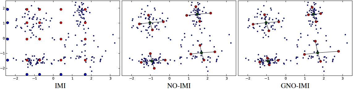
An example of indexing strategies performed on the Deep1b dataset such as Inverted Multi-Index (IMI), Non-Orthogonal Inverted Multi-Index (NO-IMI), and Generalized Non-Orthogonal Inverted Multi-Index (GNO-IMI): http://sites.skoltech.ru/compvision/noimi/
Downloading and preparing a dataset with the sheer size and dimensionality of Deep1b was challenging for a variety of reasons, each of which I will explore in detail.
The first step to benchmarking Deep1b is to download the dataset, which can be found here. Because of the size of this file, it is split into 37 “Base” files which when combined, form the complete dataset. These files are stored in “fvecs” format, a niche binary vector storage type ideal for large datasets such as Deep1b. Fvecs is structured specifically for vectors by first detailing the length of a vector as an integer (in binary), and then writing the vector dimensions as floats for the length specified by the integer. To decode this format we have to construct the file from these rules:
#Open as float32
fv = numpy.fromfile(deep1b_base_00, dtype=numpy.float32)#read the length of the vector by checking the first element
dim = fv.view(numpy.int32)[0]# reshape to a numpy array excluding the first element
fv = fv.reshape(-1, dim + 1)[:, 1:]
As we began the process of decoding the fvecs format, we ran into another issue. At some point during the 380GB download, some of our base files had corrupted. To help check against this we developed a script that checks to see if the fvecs file format is valid within the base file, and that clips any incomplete vectors from the base files. This ensures that the structure of the file is valid for conversion.
Once the base files have been validated and reshaped into NumPy arrays, we can begin the process of calculating the ground truth of the dataset and storing the file in the HDF5 format, which Bernhardsson has designed his ANN Benchmarking code around. Bernhardsson has included backup code in his project for ground truth calculations on new/altered datasets, which we will try to closely emulate. Preparing the vectors in this stage can lead to a number of memory-related issues:

Credit to Lifewire for the image: https://www.lifewire.com/troubleshooting-cf-memory-cards-493780
- NumPy uses lots of memory: One of the first issues we regularly ran into was NumPy’s memory consumption. We were pushing the limitations of our machine and had to be very careful about when and how we used NumPy for our project.
- Scikit-learn’s model_selection train_test_split function: Bernhardsson’s code for ground truth included a section for splitting the dataset with Scikit-learn’s train test split function. This continually crashed on us. As a temporary solution, we split the data in a straightforward way and will later return to a more developed memory efficient and robust solution to this problem.
- Creating the HDF5 structure: To create the HDF5 binary file format we utilized’s H5Py, a pythonic interface for the HDF5 format. Part of the memory-related challenges we faced was creating this file using such an enormous suite of data. Luckily for us, H5Py includes an auto-chunking feature for file creation. This allowed for us to seamlessly construct a complete HDF5 file without overloading memory by partitioning the data into temporary chunks for H5Py to convert.
Prepping the Benchmark
To prepare the benchmarker for a 54 million vector dataset, some quality of life improvements had to be made. Because we didn't know how long these algorithms could run for, we wanted to pepper a number of print statements throughout the project that would serve to keep track of where the algorithm was on its benchmarking journey. Furthermore, rather than run every parameter of our select algorithm, we instead chose to run our select algorithms with very basic arguments to test whether they would survive the preprocessing stage and if we could adjust them to run more efficiently. All of the algorithm parameters are stored in a YAML file type, which is a human-readable data serialization standard that functions in a variety of programming languages. This file, included in Bernhardsson’s code, allowed us to make quick changes to the various parameters each algorithm accepts. For example here is Faiss-IVF’s entry:
faiss-ivf:
      docker-tag: ann-benchmarks-faiss
      module: ann_benchmarks.algorithms.faiss
      constructor: FaissIVF
      base-args: ["@metric"]
      run-groups:
        base:
          args: [[32,64,128,256,512,1024,2048,4096,8192]]
          query-args: [[1, 5, 10, 50, 100, 200]]
There are a few key points to break down in this code. “Base-args” takes in the distance metric that the nearest neighbors should be calculated on. In the case of Deep1b, this metric is angular distance. Within the base subgroup, there are the parameters args, and query args. Args represents the number of groups the vectors are subcategorized into based on vicinity. Query-args represents the number of groups to check for the nearest neighbor. This suggests that having a high args parameter indicates a much longer preprocessing stage, and having a higher query-arg means having a much longer computation stage. Hence, args = 8192 and query-args = 200 would take the longest amount of time, but would likely have the highest recall. Different algorithms have different argument parameters and often different variables that can be adjusted to speed up, slow down, save space, or improve accuracy depending on how they are tuned. The default parameters for Bernhardsson’s project can be found here.
Running the Benchmark

Something has to go wrong, right?
After preparing the dataset and the benchmarked, it was time to begin the experiment, or so we hoped. As many readers might have guessed, our hardware limitations continued to stunt progress. Our machine, as mentioned earlier, was equipped with 64GBs of RAM, which is usually sufficient, however, in this case it was quite limiting. Many of the algorithms we have chosen to test rely on constructing large indexes to ensure fast nearest neighbor search. This can make some algorithms very time efficient at the expense of memory. HNSW(nmslib) and n2 failed while constructing the index due to memory failures.
Because we wanted to stay true to Bernhardsson’s source code, changes were not made at an algorithmic level and hence we could only benchmark algorithms that would run as cloned from Bernhardsson’s repo. Under the limitations of our system, one group of algorithms stood out. The Faiss package, which includes:
- Faiss-IVF: Inverted File Index or IVF
- Faiss-LSH: Locality Sensitive Hashing or LSH
- Faiss-HNSW: Hierarchical Navigable Small World or HNSW
Interestingly enough, Faiss-LSH was disabled by default in Bernhardsson’s code. This is likely because LSH performed very poorly when compared to its brother IVF and wasn’t worth inclusion in the default parameters of the ANN-benchmarks project.
A full list of the algorithms we tried can be seen below:

A table highlighting which algorithms we tested, their parameters, and if they failed or succeeded.
Additionally, here is a visualization of the runtime of each algorithm:
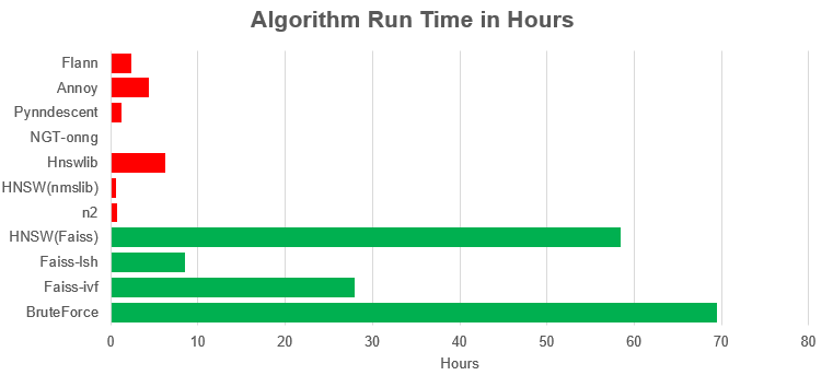
A chart highlighting the runtime of each algorithm to either failure (red) or success (green).
As you can see, many of the algorithms — with the exception of NGT which we couldn’t get to work — failed after a few hours of index construction exceeding the 64BGs of RAM our machine had available.
Finally Some Results
Given the hardware limitations, we weren’t surprised to see many of the algorithms fail in the preprocessing stage. However, it was still a surprise to see lauded implementations such as annoy fail so quickly. As it turns out, Facebook’s Faiss algorithm family is quite robust under limitations such as less than sufficient memory. Given the nature of the project, we chose not to benchmark Faiss-GPU, a nearest-neighbor algorithm provided in the Faiss library that utilizes the machine’s GPU to boost the search time and accuracy. Whilst this was feasible on our machine, it would have been an unfair advantage for that algorithm.
It is also possible that our use of the algorithms wasn’t optimal considering the scale of the dataset. We chose to emulate the conditions Bernhardsson included as default on the project as closely as possible, which could have led to us ignoring parameters that would allow these algorithms to run under low memory conditions.
With all that said, below are the results at this stage of the project:
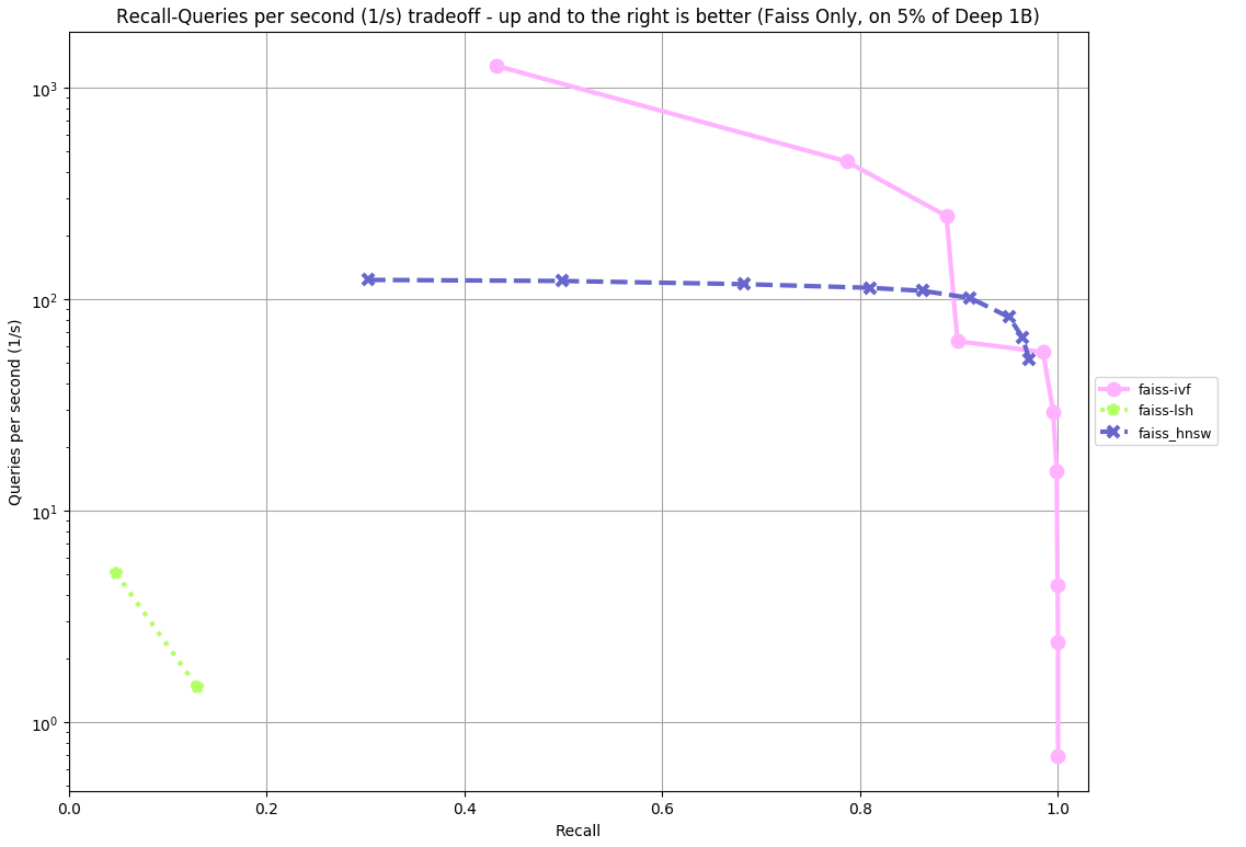
Results from benchmarking the Faiss ANN family on 5% of Deep1b
As the graph clearly indicates, Fiass-IVF greatly outperformed both of its siblings in terms of accuracy and computation time over the duration of its benchmark. Whilst LSH might have eventually reached a higher recall, it was very slow and would have likely taken a much longer time. This supports our claim that Bernhardsson had disabled LSH in favor of IVF, knowing that IVF would outperform LSH in most cases. While HNSW performed well overall, it was much slower and had a lower recall rate than Faiss-IVF, even after completing 100% of its benchmark parameters. In comparison, Faiss-IVF only completed 66% of its benchmark parameters. Though all three algorithms are impressive/noteworthy for even being able to run under the conditions of our test, it is clear that Faiss-IVF is a faster and more accurate nearest neighbor algorithm than its competing siblings.
Conclusion

In summary, this project has been a great step on the way to benchmarking the full Deep1b dataset. Running into so many issues and overcoming them has helped me gain valuable insight into some of the challenges we may face further ahead, and has also alluded to some of the more robust and effective ANN algorithms available in the world of open source. Going forward there are many improvements and changes I would like to make as we get closer to benchmarking on the full dataset. Primarily, some hardware upgrades are going to have to be made to accommodate for the sheer size of the Deep1b data set. Likely this will come in the form of some custom hardware provided by GSI Technology that will enable and speed up the whole operation. Additionally, I will have to further investigate each algorithm and optimize them for memory-constrained conditions. This will give me a better understanding of how the algorithms work and also help ensure that I am utilizing them optimally. Accomplishing both of these upgrades will help make benchmarking Deep1b a reality and highlight which ANN algorithms perform the best under the conditions of our test.
Appendix:
- Computer specifications: 1U GPU Server 1 2 Intel CD8067303535601 Xeon® Gold 5115 2 3 Kingston KSM26RD8/16HAI 16GB 2666MHz DDR4 ECC Reg CL19 DIMM 2Rx8 Hynix A IDT 4 4 Intel SSDSC2KG960G801 S4610 960GB 2.5" SSD.
- Link to the previous blog: https://www.gsitechnology.com/How-to-Benchmark-ANN-Algorithms
Sources:
- Aumüller, Martin, Erik Bernhardsson, and Alexander Faithfull. “ANN-benchmarks: A benchmarking tool for approximate nearest neighbor algorithms.” International Conference on Similarity Search and Applications. Springer, Cham, 2017.
- Collette, A. (n.d.). Python and HDF5. Retrieved July 21, 2020, from https://www.oreilly.com/library/view/python-and-hdf5/9781491944981/ch04.html
- Deep billion-scale indexing. (n.d.). Retrieved July 21, 2020, from http://sites.skoltech.ru/compvision/noimi/
- Evaluation of Approximate nearest neighbors: Large datasets. (n.d.). Retrieved July 21, 2020, from http://corpus-texmex.irisa.fr/
- Liu, Ting, et al. “An investigation of practical approximate nearest neighbor algorithms.” Advances in neural information processing systems. 2005.
- Malkov, Yury, et al. “Approximate nearest neighbor algorithm based on navigable small-world graphs.” Information Systems 45 (2014): 61–68.
- Laarhoven, Thijs. “Graph-based time-space trade-offs for approximate near neighbors.” arXiv preprint arXiv:1712.03158 (2017).