20,000 Signals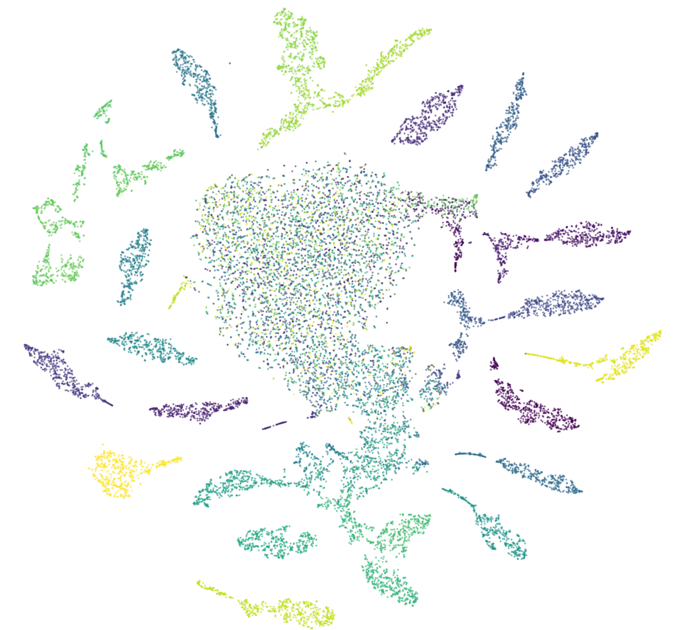
Last Time
In my last blog, I described how I built a radio wave classifier in Python. We trained a deep residual neural network to classify 24 different classes of radio waves that are used in satellite communication. It turns out that with a slight tweak to the network we built, we can turn radio signal classification into a similarity search problem.
Similarity Search
Recall from my blog on similarity search how we built up a notion of distance as it relates to similarity. To reuse an example, imagine you conduct a survey and record the height and weight of ten people. We will refer to height and weight as features. By plotting out the data points, you will notice that some data points are plotted closer together because the individuals have a more similar height and weight measurements.
Height vs. Weight Graph
As you can see in the graph above, Shivang is most similar to Jay, Leon, and Dan since they are the closest data points.
In a similar way, we can use neural networks to extract abstract features from signal data. And, as we will see, we can use these feature embeddings to ultimately classify signals.
Neural Network Embeddings
A neural network embedding is a learned continuous vector representation of data. By extracting an embedding from signal data, we are essentially mapping signal data to unique points in n-dimensional space.
Here’s the ResNet architecture that was used to train my signal classifier: 2x1024 dimensional signal data is entered through the model as input and the output is a 24 dimensional list of probabilities associated with each signal class.
ResNet Architecture
Notice that we make only one small change to our previous architecture — We add a 50 dimensional dense layer just before the final output layer. This 50 dimensional dense layer will serve as our embedding layer.
Let’s take a closer look at the embedding layer:
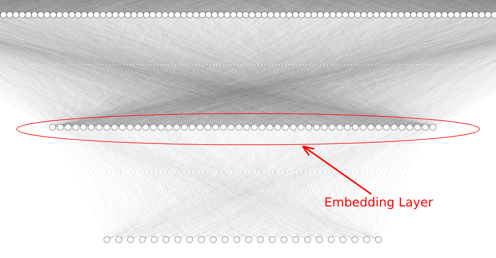
Embedding Layer
We apply a Sigmoid activation function to each individual node of our embedding layer. The output of the Sigmoid function is a decimal value between 0 and 1.

Sigmoid Activation Function
This function is chosen for its unique properties: very large positive inputs will be mapped very close to one and very large negative inputs will be mapped very close to zero.
If we enter data for some signal into our model, we can extract the output of the model at the embedding layer — The result is a list of 50 numbers between zero and one. The embedding output may look something like this:
[0.5, 0.018, 0.269, 0.007, 0.119, 0.269, 0.953, 0.953, 0.269, 0.881, 0.018, 0.047, 0.047, 0.047, 0.007, 0.018, 0.018, 0.982, 0.047, 0.047, 0.881, 0.047, 0.953, 0.881, 0.881, 0.982, 0.953, 0.731, 0.269, 0.982, 0.5, 0.731, 0.018, 0.269, 0.5, 0.881, 0.119, 0.881, 0.731, 0.5, 0.881, 0.119, 0.119, 0.047, 0.018, 0.881, 0.047, 0.007, 0.119, 0.269]
Visualizing the Embeddings
Similarly to the height and weight example from earlier, we can plot out the embedding features to get a visual notion of similarity. The only problem, however, is that our extracted feature vectors are 50-dimensional. It is very easy to visualize a simple 2D plot from the height and weight data, but we are unable to grasp a meaningful concept of any visualization beyond the third dimension.
The solution to this is a dimensionality reduction algorithm called t-SNE. This algorithm allows us to project our signal embedding data in a 2D grid in such a way that the original clustering from 50-dimensional space is preserved.
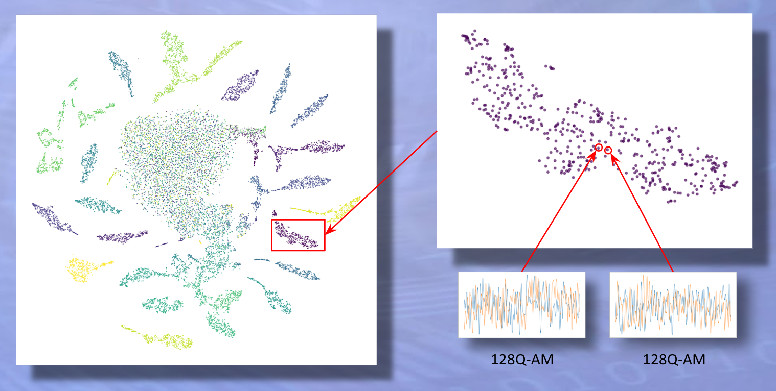
Clean signals cluster together by radio wave class. Notice the two signals close to each other are of the same class. In this case, 128Q-AM.
In the above image, we have plotted out the data points for 20,000 different radio signals. Data points that are the same color belong to the same class of signal.
Notice the distinct clusters of data points that formed. Signal embeddings of the same class are clustered together. We can take advantage of this for classification purposes.
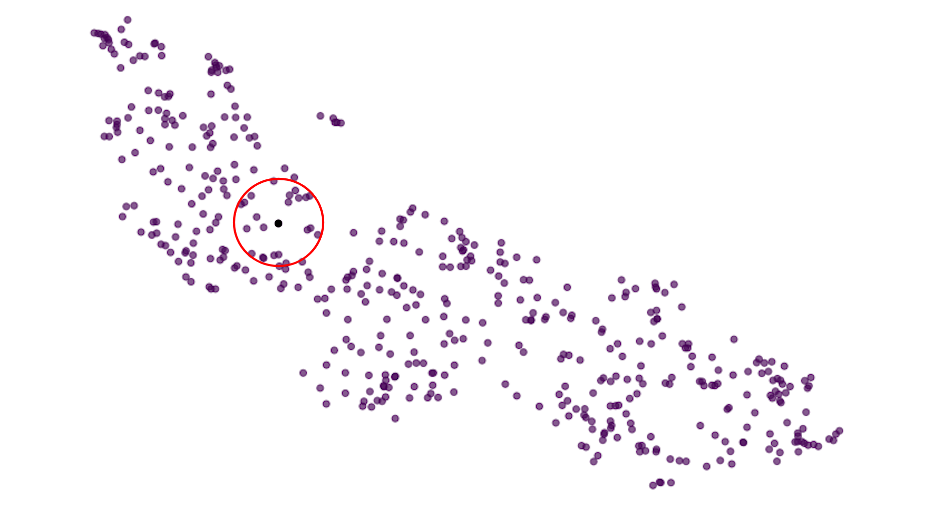
Specific signal classes cluster together
The idea being that, if you randomly select some datapoint whose signal class you do not know, you can infer the class of that datapoint based on the data points that immediately surround it.
If all the signals surrounding our random datapoint are AM signals, we can assume with some confidence that our random datapoint is also and AM signal.
But what about the big blob of speckled, mixed data points in the middle of the graph?
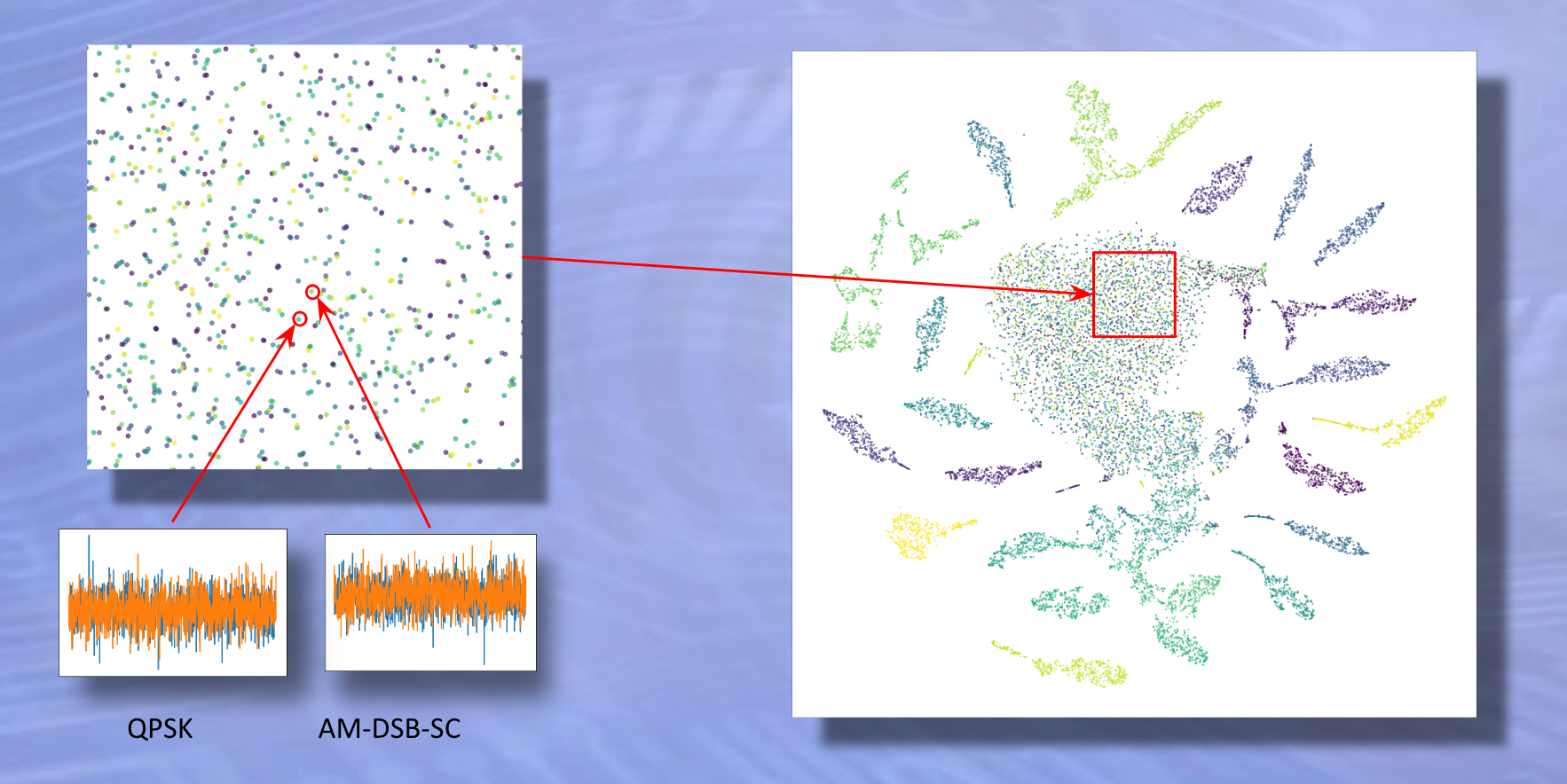
Noisy, unrecognizable signals blob together in the middle.
Taking a closer look at the data points in the center cluster, we can see two examples that look very similar but are from two different signal classes. This is because a high amount of noise is present in both signals.
The algorithm has a hard time clustering these points into tight groups because the signals are virtually unidentifiable.
The problem with finding all the nearest neighbors for a given data point is that there is a high computational cost associated with calculating Euclidean distance between high dimensional vectors. Luckily, we can speed up the search process with a small but clever trick …
Binary Fingerprints for Radio Signals
Instead of calculating Euclidean distance between our embeddings, we will convert our embeddings to bit vector fingerprints and compare similarity using another metric called Hamming distance.
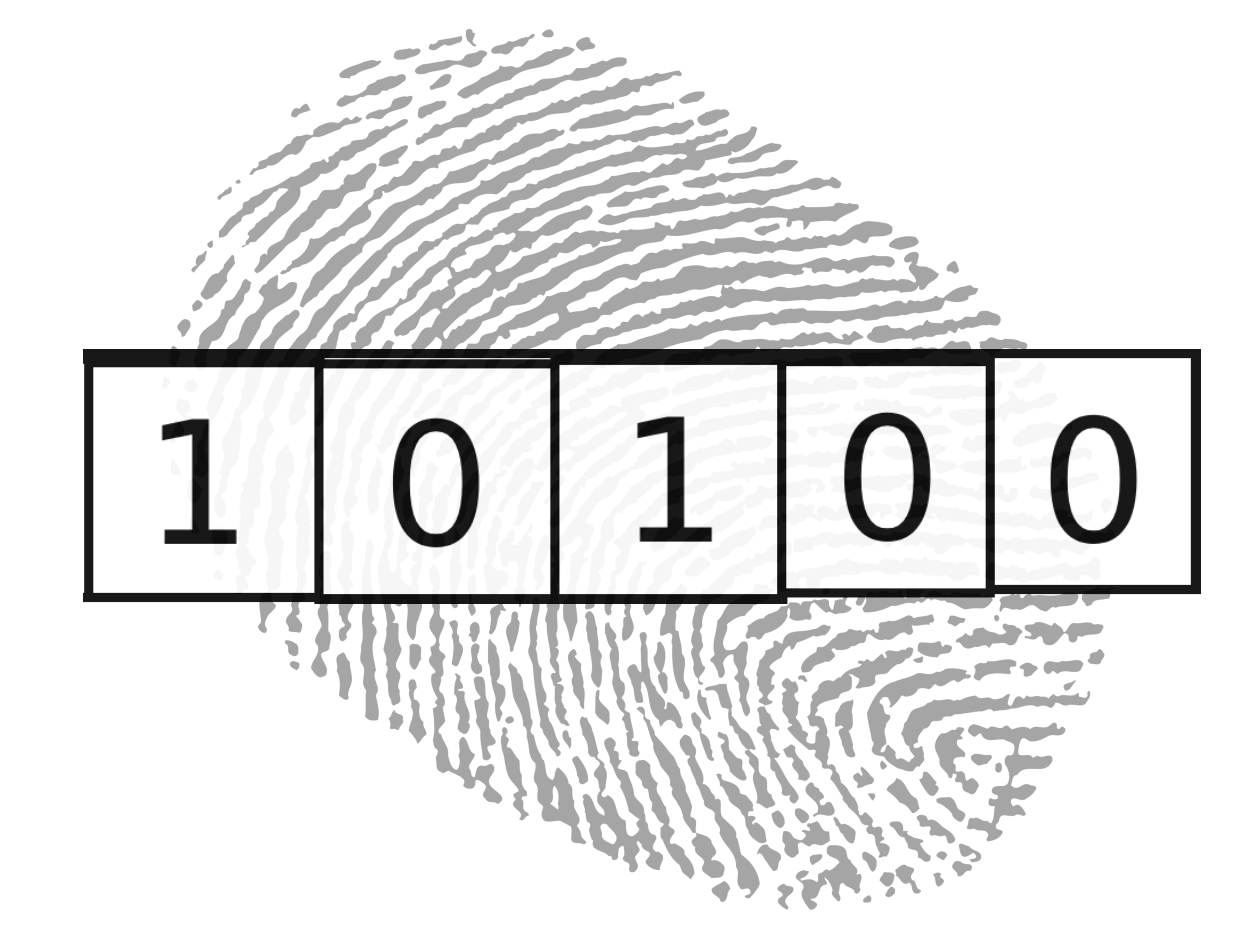
To convert an embedding vector to a bit vector fingerprint we do the following: if a node is greater than .5, we set the node equal to 1. If a node is less than .5, we set the node equal to zero. That’s it!
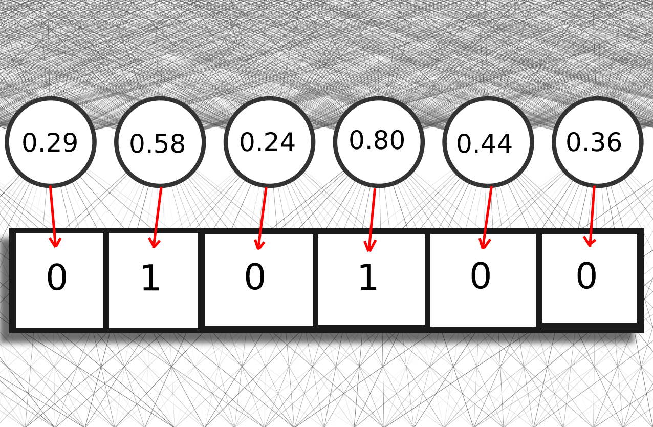
Turning an embedding into a bit-vector
A great benefit to this approach is that there is a much lower memory cost associated with bit vectors compared to the original signal data which is floating point.
Computing the hamming distance between two binary fingerprints is very simple and very fast. To compute the Hamming distance between two bit vectors, we count the total number of times that corresponding values are different.
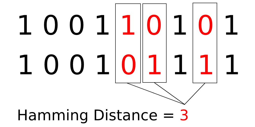
Hamming distance calculation
The Hamming distance between the two fingerprints in the above example is three because there are three corresponding values that are not equal.
k-Nearest Neighbors Search
Now suppose you have a signal that you would like to identify. We will call this our query signal. Then all we would need to do is get the binary fingerprint for the query signal using the process described in the previous section and then search against a fingerprint database of known signals. We are looking for other signals that have the smallest distances to our query signal.
For my experiment, I chose k = 5. This means that we search for the top five signals (i.e. nearest neighbors) in our database that have the lowest Hamming distance to our query vector.
If the majority of the 5 nearest neighbors are from a particular class, we can safely assume that the query signal also belongs to that class.
Evaluating Performance
To see how well the similarity search classification method performs, I compare it with the original ResNet classifier from my previous blog. I also compare how the length of the bit vector affects classification accuracy, examining bit vectors fingerprints of lengths 20, 50, 100, and 500.
Let’s talk about what this plot means.

Each signal class is composed of many examples with different amounts of noise present. The cleaner signals have the highest signal to noise ratio and are thus easier to classify for the ResNet and k-NN similarity search. As the signal to noise ratio decreases, the accuracy goes down.
Notice that the accuracy for all the techniques shown are roughly the same except for bit vector size = 20. Intuitively this makes sense because 20 bits is too small of a representative feature space for all the signal types. But also notice that there is no benefit beyond a bit size of 50.
Conclusion
One of the great benefits to this approach is the huge savings in memory storage. Our original signals are stored as 2x1024 dimensional floating point data. Each signal requires 65536 bits of memory. Compare this to the 50 bit fingerprints that we generated. Our bit vector requires 99.99% less memory than the original signal.
The interesting question at hand is if we can use this model as a feature extractor for broader classes of signals that have not been seen during training. This method is called transfer learning and we will explore this more in future blogs.
We are also looking forward to running experiments on GSI’s new Gemini APU chip which is optimized for similarity search applications like signal classification.
Code
Here is a link to my code implementation for anyone interested in doing their own experiment with embeddings or similarity search.
Neural Network with Embedding Layer, Similarity Search Classifier