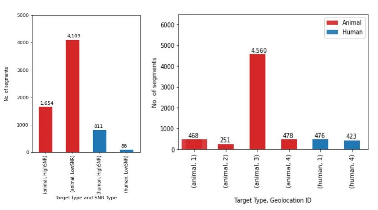
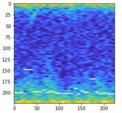
The Israeli Ministry of Defense’s R&D Directorate (MAFAT) launched a fascinating challenge on July 15th, 2020, with the goal of the challenge being able to distinguish between humans and animals in radar signal segments. This article will attempt to share the core of our solution that was awarded the first-place prize and the most significant ideas and challenges this competition presented, and how we approached them. It was a very rewarding experience, and we would like to thank the MAFAT team for the opportunity and for the well-structured material and informative resources they provided to the contestants. Final challenge results. Image from competition site. The challenge was to distinguish between animals and humans in short segments acquired by doppler-pulse Radar Systems. The segments are taken from real world radar tracks of animals and humans detected by different sensors at different locations, terrains, and Signal-to-Noise Ratio (SNR). Each segment is defined using a 128 x 32 I/Q matrix — a complex number representation of the received signals over 32 time units and a doppler burst vector, representing the object’s center of mass. The organizers also supplied a method for modelling the I/Q matrix into a spectrogram — which is a visual representation of the spectrum of frequencies of signals over time. Simplified, the X dimension of a spectrogram can be considered as time and the Y dimension as the frequency + phase (in a single phase parameter). Example tracks of Animal/Human with High/Low SNR represented as a spectrogram image. The doppler burst readings have been added in white. Images provided by MAFAT. Reposted with Author’s permission. The differences between an animal and a human in such images lie in the micro-doppler signals of the non-rigid objects, created mainly by the movement of the limbs (i.e., arms, legs, and tail), though to an untrained eye it seems impossible to understand or classify such images. The segments indeed contain information of the target object, but also of signal noise and of clutter — signals received from the existing background environment such as grass, trees or weather conditions. A main challenge was to extract target-relevant features from the spectrogram and avoid incorporating background and noise into the decision. The organizers also supplied useful auxiliary data — mainly experimental human tracks in some locations, synthetically created noise added to originally high signaled segments, to simulate low SNR, and background-only segments in several locations, that do not include any objects. For a more detailed description, insights into the data and references — we recommend reading the previous article posted by GSI Technology and visiting the challenge site. The training and auxiliary data included metadata providing each segment with a unique ID, a track ID, sensor ID, geolocation, geolocation type (terrain), SNR type (high/low/synth), calendar day, and finally, target type (human/animal). A notebook provided by the organizers gave a thorough statistical analysis of the data, enabling us to attain some key insights: Descriptive statistics produced by MAFAT’s notebook. It was obvious the solution would have to tackle these challenges — to somehow balance the data, to avoid learning features of the environment and image quality, rather than the features of the targets themselves and to manage to extrapolate well from the training data onto the test data. Who doesn’t like a good cats vs. dogs analogy? Image by Free-Photos from Pixabay As we had no prior experience in radar systems or signals, we first familiarized ourselves on the subject. Luckily, the competition organizers provided very informative explanations, and reading them, along with a short online research on the subject, was enough to start working on the project. Additionally, we searched online for relevant work or papers on classification of spectrograms from doppler signals. We found very few works out there. Mainly we found one work that models a hybrid 1D-CNN /RNN network to classify human activities from doppler signals, and another that distinguishes drones from birds, comparing results on RGB vs. Gray input images and of pretrained GoogleNet model vs. custom serial architecture. In both cases, the data seemed quite different (diverse, cleaner, with longer segments), and it seemed clear that a unique solution would be needed for this challenge. To add more human samples and low-SNR samples, the experiment and synthetic SNR sets, included in the supplied auxiliary data, were added to the original training set. Still, the highly unbalanced data, as reviewed above, presented difficulty in achieving a good generalization from the training data onto the test data. Random training-validation splits were not an option if we wanted to reflect the results on the test set from the validation set, for efficient monitoring of the development process. Thus, a careful selection of a split was performed and maintained constant throughout the development, until a steady solution was achieved, at which point the split was neglected and the entire data was used for training. Decisions over the split selection were based mainly on geolocations, trying to keep a large “same-environment, different target” (e.g., geolocations 1 & 4) group for training, and “new-environments, still versatile” group for validating. To further cope with the unbalanced data during training, in each epoch — up to three segments-per-track were randomly selected from the training split (a slightly different approach to up-sampling small tracks) and in each training batch — an equal amount of human and animal segments were selected, promising a balanced loss during the training process. The challenge’s evaluation metric was AUC, but it did not prove robust for evaluating the solution on the different validation sets, as it constantly produced high accuracy and neglected consideration of unbalanced validation sets, consequently failing to reflect results on the test set. Therefore, the evaluation metric we used to monitor the training process during development was balanced accuracy, defined as: If coping with the unbalanced, scarce data distribution was one main challenge to consider, the representation and pre-processing that the data should go through before fed into a classifier, was the other. Should it be the raw I/Q matrix? The modeled spectrogram created with the provided conversion scheme? Maybe a different method? And should it be the complex number representation? Absolute value (phase)? Or the RGB heatmap? Perhaps a mixture of the above? And how, if at all, should the center of mass be included? As a white overlay to the spectrogram or as an independent vector? Considering the small training data and after experimenting with a few of the above, we decided it best to simulate as much resemblance to pretrained information of images from existing models and thus use the visual spectrogram in RGB format, with the center of mass overlaid on top in white, and the entire image resized to 224 x 224 pixels. Example pre-processed input segment. Image by author. Though the spectrograms are far from being natural images like in ImageNet, maintaining initial models’ feature extraction from the basic shapes and patterns seemed to come in handy. A key addition, providing a large boost in accuracy, were the data augmentations to the training set. a) Most importantly, in order to combat the risk of learning background features, the model was “challenged” with segments “corrupted” by random background segments from the auxiliary set. The corruption was done mainly in the original I/Q space by adding/subtracting background-segments to the original segments by a random factor. Additional augmentations were performed on the visual spectrograms and included: b) Horizontal and vertical flips. Flipping the time and phase dimensions of a spectrogram may not be intuitive, but it maintained categorical information and offered good augmentation. c) Wrapped vertical translation. Since the Y axis represents a cyclic phase, a random cyclic translation was performed on each spectrogram, meaning the shifted data was reassigned in a cyclic manner. The translation was uniformly random over the entire y-axis so that frequency relations and patterns where kept, but no absolute values (supposing it can be considered as fast-forwarding/slow-motion). d) Cross-track horizontal translation. The segments divide each track in a constant manner, but more segments can be created from a track by moving the segment windows left or right by a few pixels within a track. e) Finally, predictions of several (six, to be exact) test-time-augmentations were averaged to create the final prediction. Different augmentation examples on an original segment (first on the left). First two present random background augmentations. Next five examples are horizontal and vertical flips and three wrapped vertical translations. Images by Author. Several public CNN models were evaluated and included in the final prediction, most notably ResNet, DenseNet, and EfficientNet, all initialized with ImageNet pretrained weights. Each architecture went through different training stages, where a different number of layers were “released” for training (unfrozen) and the learning rate was modified (hint— not necessarily in one direction). Hybrid models with 1D convolutions and recurrent layers were also investigated but at the time of submission did not prove competitiveness to the standard CNNs. Admittedly, due to time limitations (as we entered this competition rather late), little effort was invested into the ensembling process and into decorrelating the trained models. Eventually, a mixture of 33 models were involved in the ensemble, with the difference between them being the initial weights, the random balancing/augmentation and the architecture (Resnet50, DenseNet, EfficientNets B3/4/5). The winning entry was a weighted ensemble, with the weights trained on the public test set using a Differential Evolution optimization scheme. The ensembling provided a further ~1% accuracy over a single model on the public test set. This was a very rewarding experience! And not just because we won :) We still have a lot of ideas for further improvements and anticipate the next challenge!

The Challenge

The Data
To a “computer visionist”, these may be analogous to learning from very few, low-quality images of cats as opposed to many high-quality images of dogs, and from mainly images of dogs at the park, while images of cats are mostly indoor… a test image of a cat at the park may very well confuse the trained classifier in such a case.
Thankfully, the provided auxiliary data included synthetically produced low-SNR segments, experimental human tracks from three new geolocations, and background-only segments from several locations — all of which proving to be very useful in the final solution.

Our Approach
Training-Validation Split
Data Balancing
Evaluation Metric
0.5*TP/(TP+FN) + 0.5* TN/(TN+FP), with Negatives (0) being animals and Positives (1) humans, and classification performed by thresholding prediction at 0.5.
Pre-Processing
Data Augmentations

Models
Ensembling
Final Words and Insights
This project offered a rare glimpse into the world of radar signals, and their challenges and proved that these challenges can be tackled without vast domain knowledge or expertise. It’s very interesting to see how — if you know how to visualize and manipulate the data well enough — a seemingly abstract representation, uninterpretable by the inexperienced eye, can be solved using classic CNN models.
References