Signal 
Signals Are Everywhere!
You can’t see them, but there are signals everywhere — A signal is an observable change in quantity that carries information. A signal can carry information about virtually anything from audio to video and text data. The ability to classify signals is an important task that holds opportunity for many different applications. For example, EMG sensors measure electrical activity in response to nerve stimulation of the muscle. If EMG sensors are attached to the wrist, electrical signals can be classified as individual finger movements which can then be used to control a robotic hand.
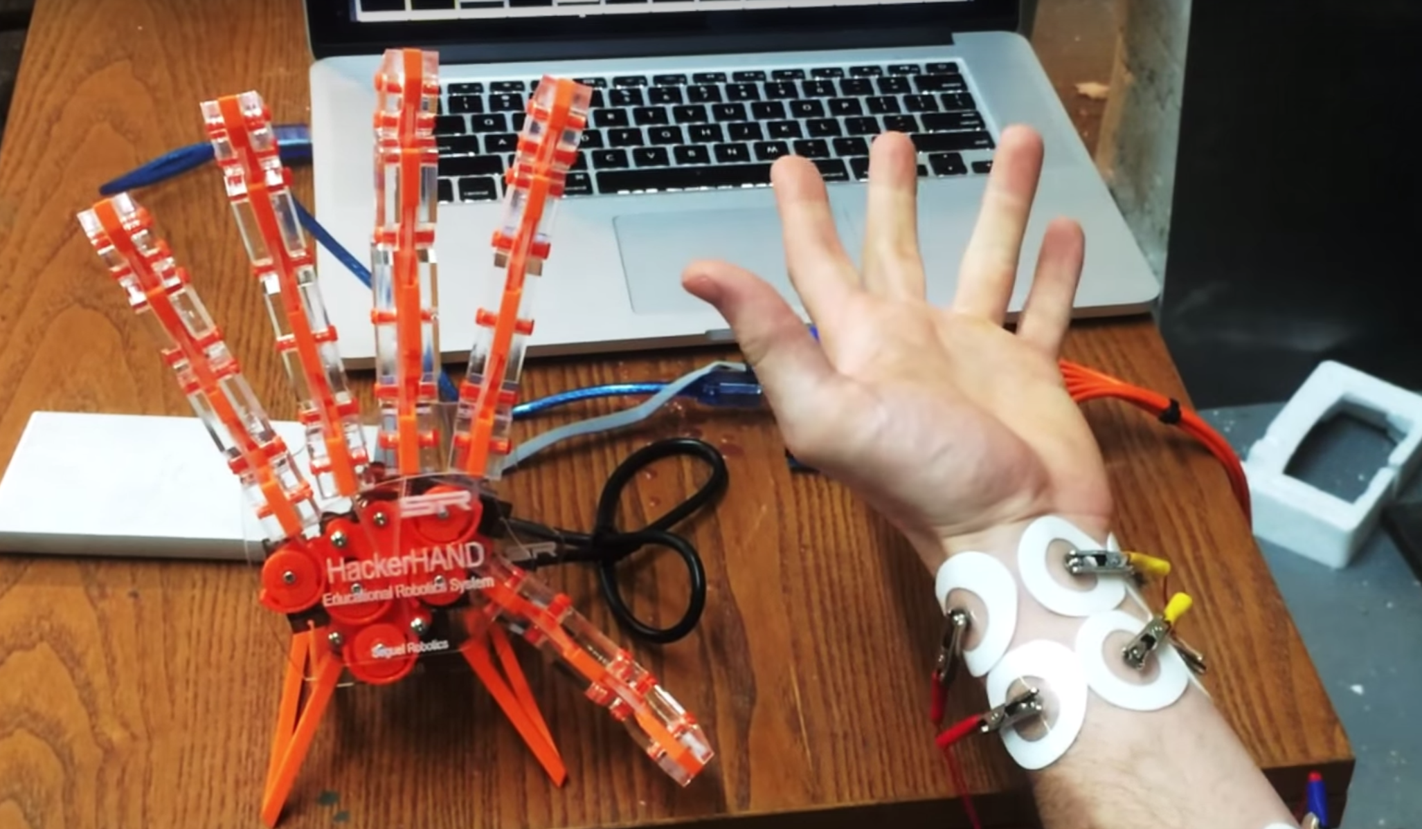
Signal Classification to Control Robotic Hand
Because there are so many different kinds of signals, we need a way to differentiate and extract information from signals. This is a topic that my mentor asked me to explore as part of my summer internship at GSI Technology, specifically regarding radio signal classification.
The Wireless Revolution
The existence of radio waves was successfully proven in 1888 by German physicist Heinrich Hertz. Only six years after the discovery, Gugliemo Marconi began developing the first wireless radio telegraph, kicking off a revolution in wireless communication. The importance of radio waves in the way our modern world functions cannot be overstated.
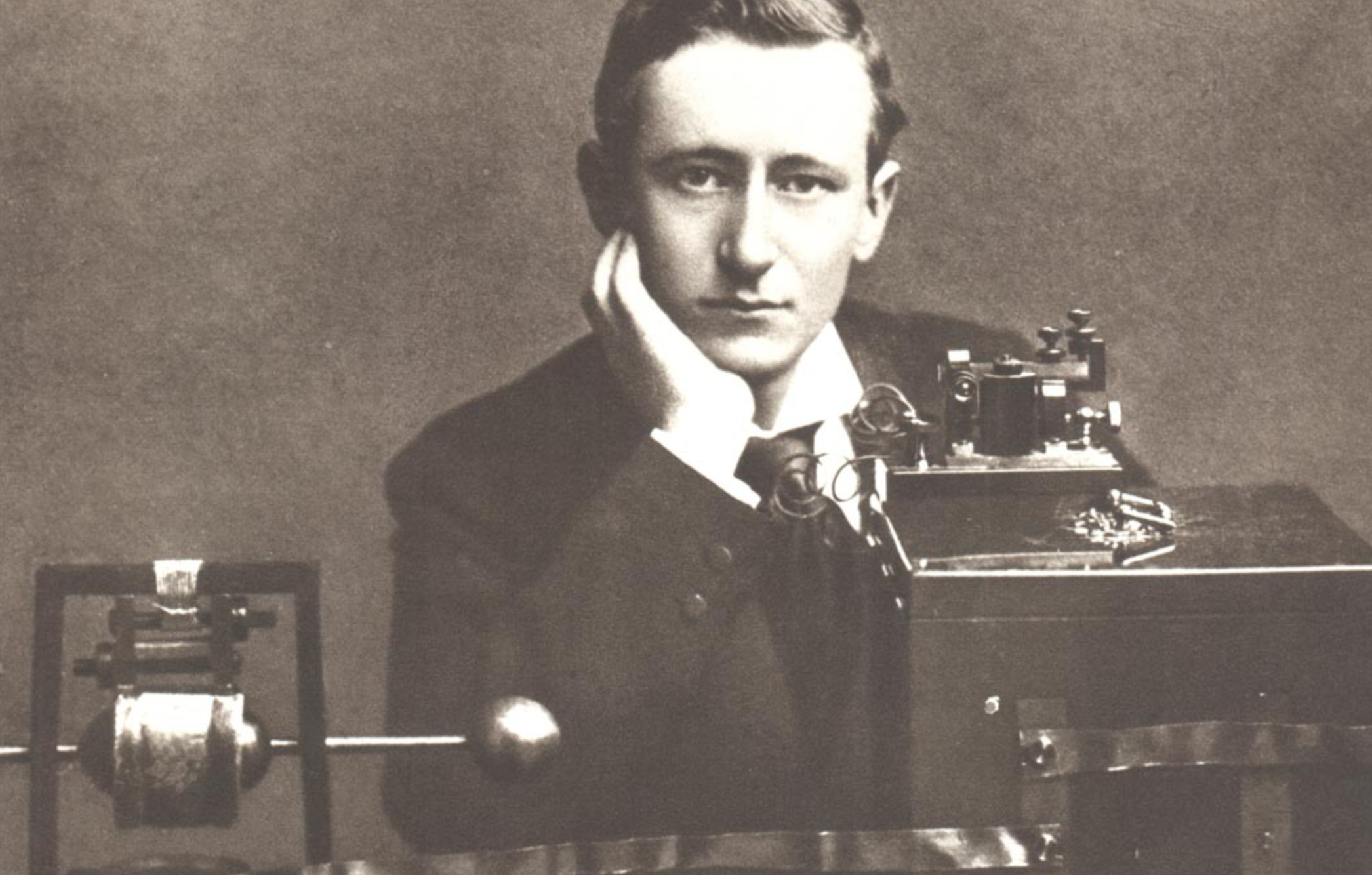
Gugliemo Marconi (1874–1937), Engineer and Physicist
In an age of mass wireless communication, the need for fast and accurate electromagnetic signal processing has never been greater.
Many different parties share the RF spectrum. A key technique for spectrum monitoring and mangagement is signal classification. We need to quickly differentiate and identify signals right off the antenna.
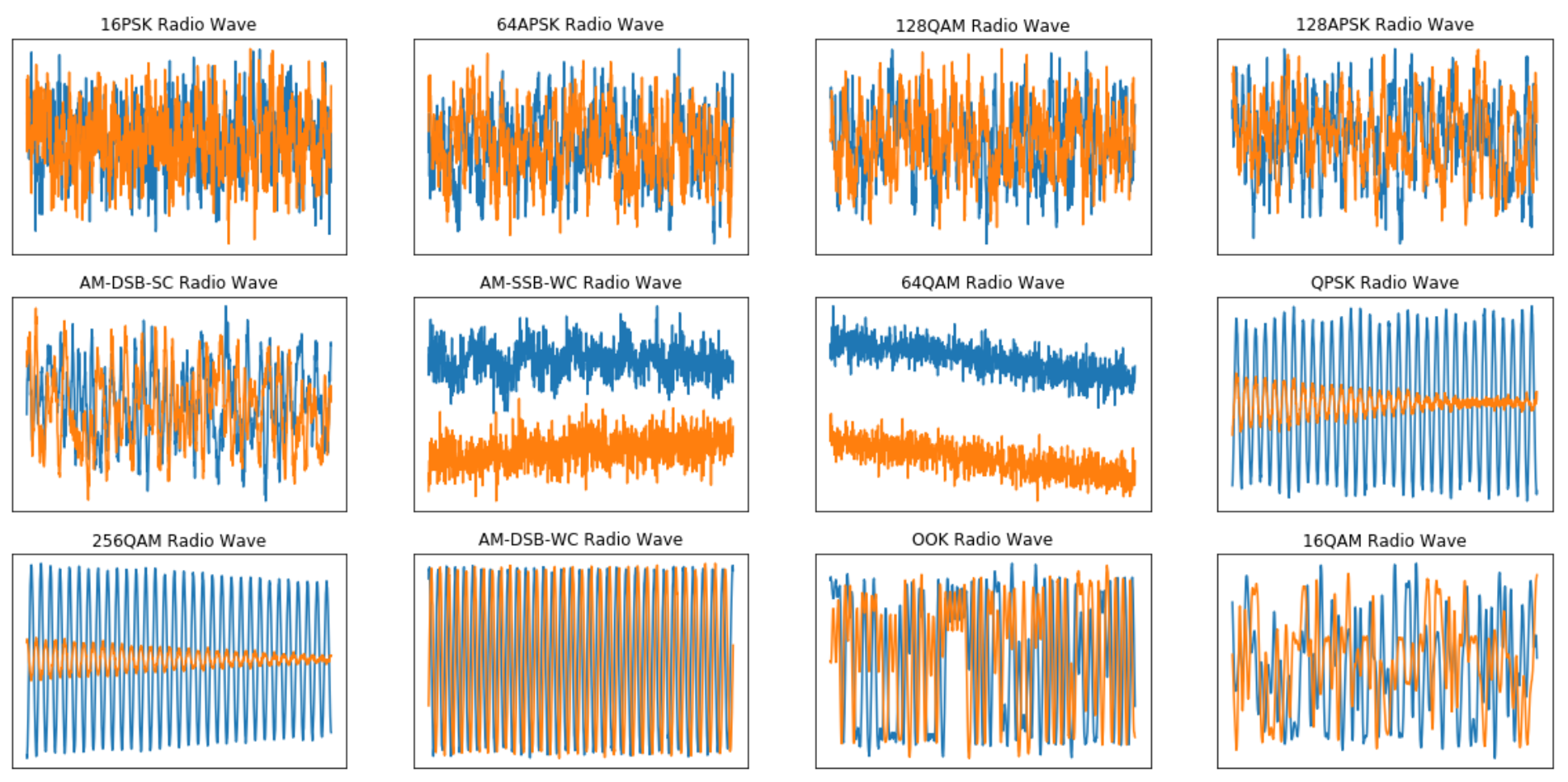
Examples from the DeepSig RADIOML
In a typical RF setting, a device may need to quickly ascertain the type of signal it is receiving. Consider the image above: these are just a few of the many possible signals that a machine may need to differentiate.
It turns out you can use state of the art machine learning for this type of classification. But first let’s take a look at the traditional method for signal processing.
Fourier Transforms
Jean-Baptiste Joseph Fourier (21 March 1768–16 May 1830) was a French mathematician and physicist best known for discovering the Fourier series and Fourier transform, the basis of all theories involving signals.

Jean-Baptiste Joseph Fourier: A Stylin’ Dude from the 1700s
The basic idea behind Fourier transforms is simple and best described by an analogy: if a painter mixes several different colors together, find the original recipe of colors that created the mix.
Instead of mixed paint, however, we want to find the recipe that makes up a given signal reading. The Fourier Transform reverse engineers a given signal in order to find all the different frequencies that comprise it.
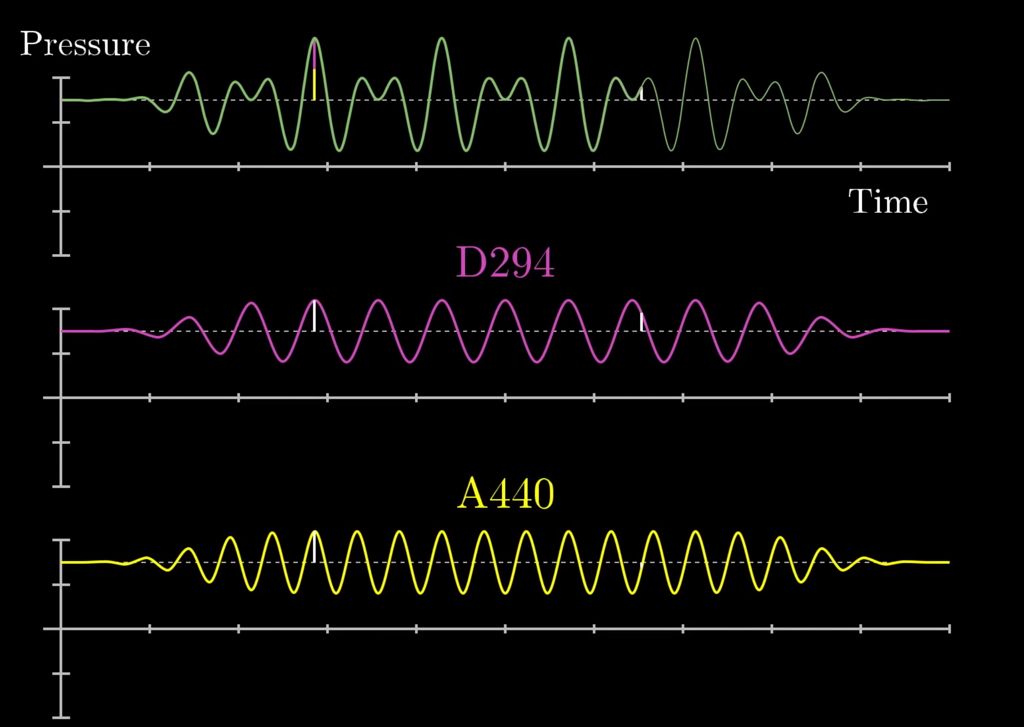
The audio signal in green is decomposed into its component notes below it. “D294” is the D note at 294 Hz. “A440” is the A note at 440 Hz.
Consider the image above, an example from the domain of sound. When you combine the yellow and purple frequencies together the result is the green signal at the top. The Fourier transform is a mathematical function that can be used to show the different frequency components of a continuous signal .
How Does it Work?
To illustrate how the Fourier transform works, let’s consider a simple example of two sinusoidal functions: f(t) = sin(2t) and g(t) = sin(3t).

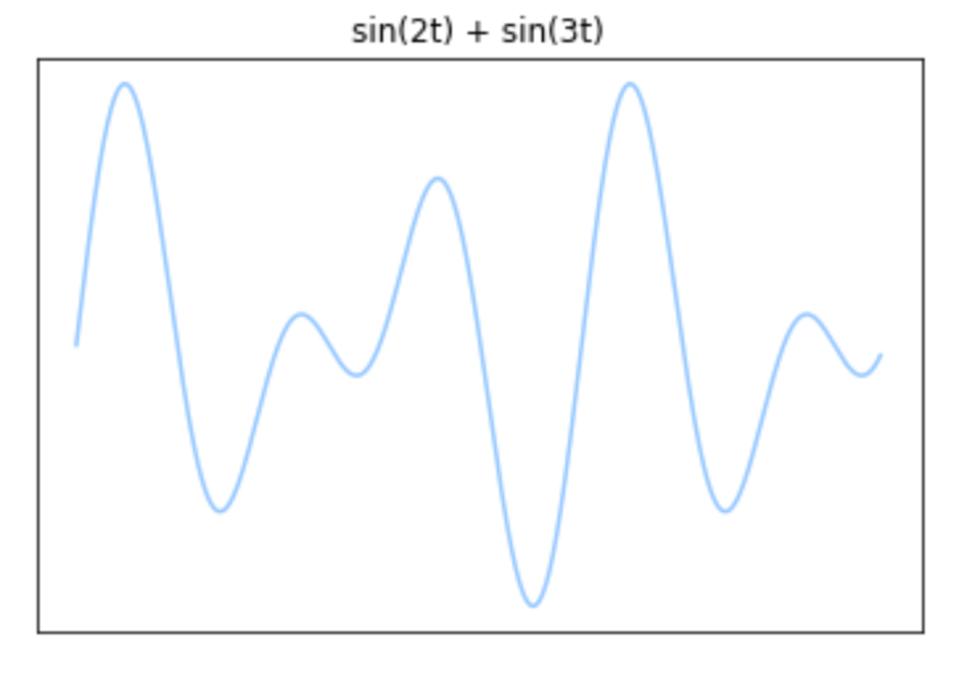
Adding the blue and green frequencies (left image) results in a combined wave (right image).
Imagine if you were just given the signal on the right; how could you decompose it into its original two components shown on the left?
A Fourier transform will help us do this. It translates signals in the time domain to the frequency domain. So after applying the transform to the signal on the right you would get something like this:
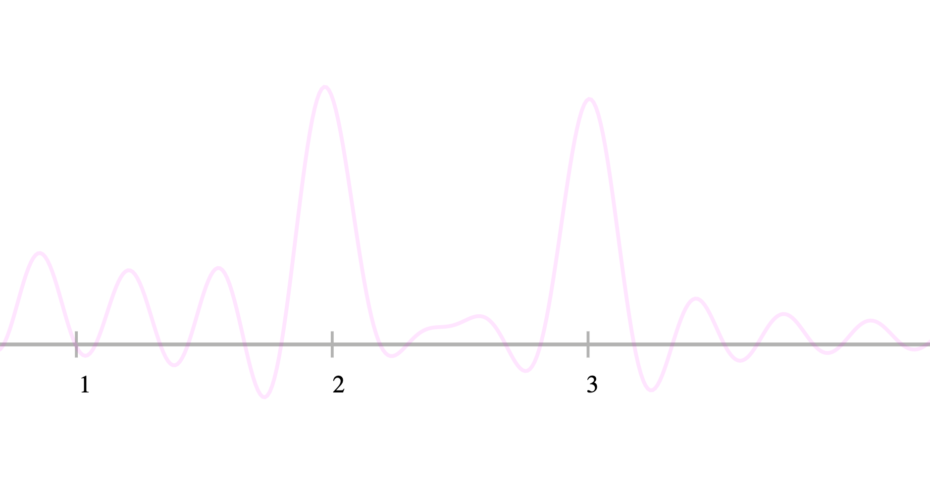
The x-axis is frequency. Notice the distinct humps over f = 2 and f = 3, the coefficients of the original component sinusoidal functions!
Now let’s look at how to do all of this in Python.
Generating Signal Data
Here we generate two sinusoidal frequencies sin(2t) and sin(3t).
# frequency, in cycles per second, or Hertz
f1 = 2
f2 = 3# sampling rate, or number of measurements per second
sample_rate = 100
seconds = 10
intervals = seconds * sample_rate# create signal time series data
t = np.linspace(0, seconds, intervals)
sin1 = np.sin(f1 * 2 * np.pi * t)
sin2 = np.sin(f2 * 2 * np.pi * t)
Then we plot out the frequencies …
# plot signal
plt.plot(t, x1)
plt.plot(t, x2)
plt.xlim(0,2)
plt.title('sin(2t) and sin(3t)')
plt.xticks([], [])
plt.yticks([], [])
plt.show()
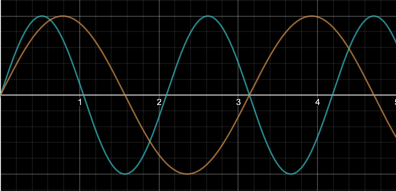
sin(2t) and sin(3t)
Generate and Plot the Signal
Here we add sin(2t) and sin(3t) together to generate our combined signal:
# generate signal
signal = []
for i in range(len(sin1)):
    signal.append(sin1[i] + sin2[i])

# plot signal
plt.plot(t, signal)
plt.xlim(0,2)
plt.title('Combined Signal')
plt.xticks([], [])
plt.yticks([], [])
plt.show()
And we plot the result:
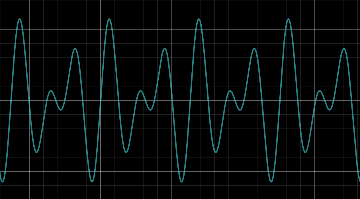
sin(2t) + sin(3t)
Fast Fourier Transform (FFT)
Now we will apply a fast Fourier transform to our signal above using a built in function from the SciPy Python library:
signal_fft = fftpack.fft(signal)
signal_fft = np.abs(signal_fft)
freqs = fftpack.fftfreq(len(signal)) * sample_rate# plot fft
plt.plot(freqs, signal_fft)
plt.xlim(0,5)
plt.style.use(['dark_background'])
plt.yticks([], [])
plt.show()
And by plotting out the result we get this:
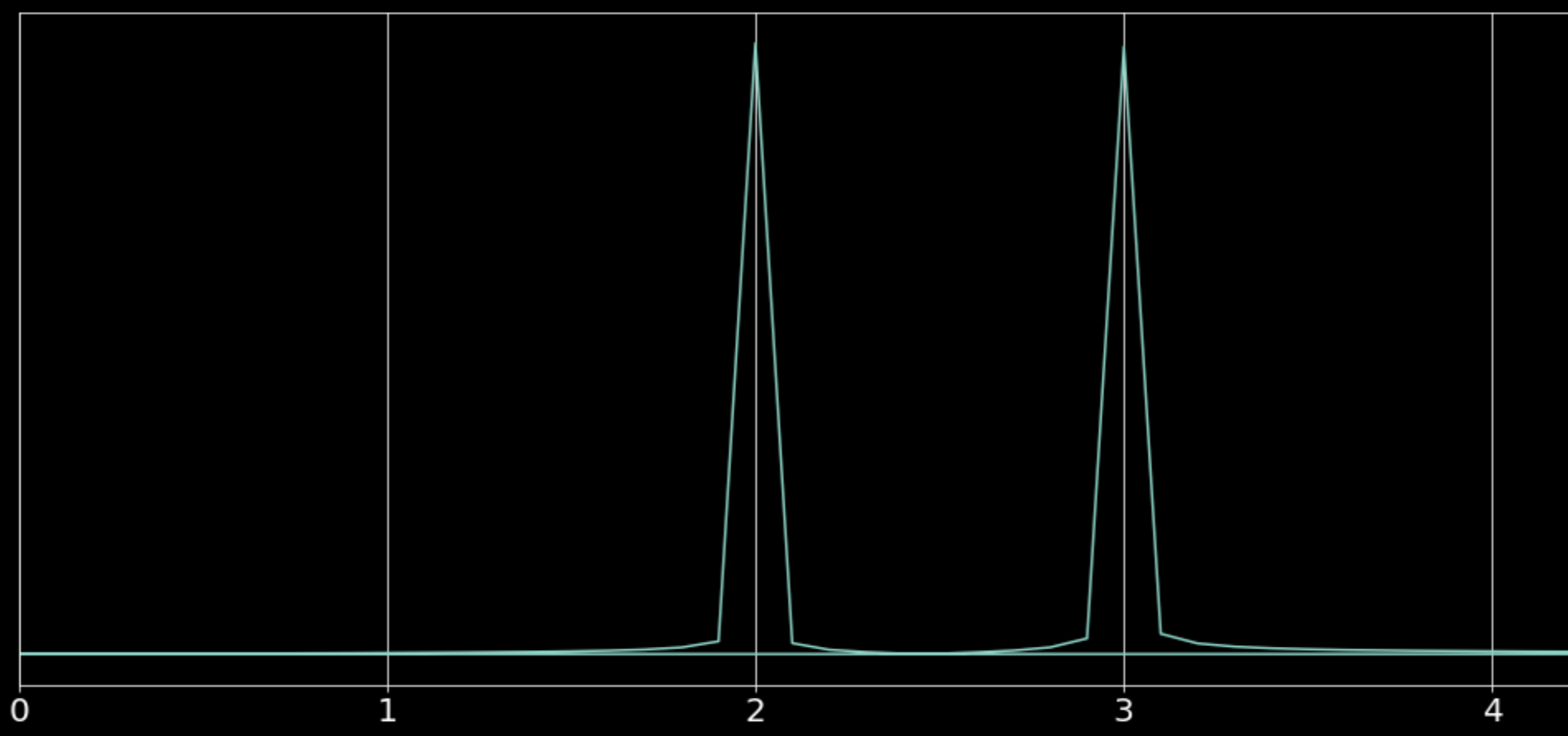
Fast Fourier Transform on Figure 1 (Frequency in Hz)
Notice how all the values of FFT are close to zero except around the frequencies 2 and 3, i.e., the frequencies corresponding with sin(2t) and sin(3t). We successfully isolated the fundamental frequency components of the signal. The Fourier transform takes a signal from the time domain to the frequency domain.
Some of you might notice that the diagram above is slightly different than that illustrated in Figure 1. This is because Figure 1 is the continuous Fourier transform and the one above is a FFT, which is much faster but also discrete and approximate.
This is intended to be a very brief introduction to the Fourier transform. If you want to learn more on this topic I recommend watching 3Blue1Brown’s video: But What is the Fourier Transform.
A Deep Learning Based Approach
Fourier analysis has been the dominant mathematical technique for processing, deconstructing, and ultimately classifying signals. But more recently, there is increased interest in using deep neural networks to accomplish these tasks.
Lately I have been experimenting with convolutional neural networks to classify radio signals from a small dataset with 11 classes. I used the simple CNN architecture shown below:
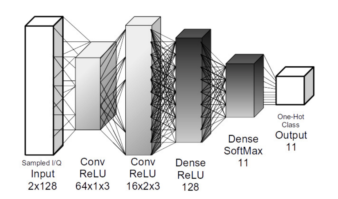
Convolutional Neural Network Architecture
The convolutional classifier reached up to 73% test accuracy.
Deep residual networks (resNets) have demonstrated state of the art results in image and audio processing and show promise for signal classification. I will try using a deep residual network on a much larger database of radio signals with even more classes of signals. In my next blog, we will look into an interesting paper that experiments with using residual neural networks for signal classification.