
Introduction
In my last blog I summarized a research paper that investigated the use of residual neural networks for the purposes of radio signal classification.
In this blog I will get you started with Google Cloud Platform and show you how to build a ResNet signal classifier in Python with Keras. Here is a link to my GitHub with the ResNet code: GitHub.
This blog is broken up into four parts:
♦ Introduction to Google Colaboratory
♦ Setting up a virtual machine instance with a Tesla V100 GPU
♦ Connecting a Colab Notebook to a virtual machine in the cloud
♦ Coding and training a ResNet in Python with Keras from scratch
Part I: Google Colab Setup
The authors of the paper include a link to the dataset that was used in the experiment so we can conduct our own experiments and training sessions. I will walk you through my experience coding a ResNet and reproducing the experiment from the paper.
Getting Started
Before we code and train a ResNet something must be considered: A lot of data means a lot of training time — I initially started training my ResNet model on my 2015 Macbook Pro with an Intel i5 processor. Each epoch took approximately 3 hours to complete on a one-million signal data base… Not ideal when planning on training for over 100 epochs. Luckily, Google provides a convenient (and free) solution to speed up the process:
What is Google Colaboratory?
Google Colaboratory is a free Jupyter Notebook setup that is entirely cloud based, accessed through your browser, and super easy to start using immediately. No need to download Python, Jupyter Lab, or install common machine learning libraries — the environment comes pre-configured for our deep learning needs out-of-the-box. Google Colab will allow us to write and execute Jupyter Notebooks directly in the browser with an attractive and intuitive user interface.
- Go to Google Colab and click NEW PYTHON 3 NOTEBOOK.
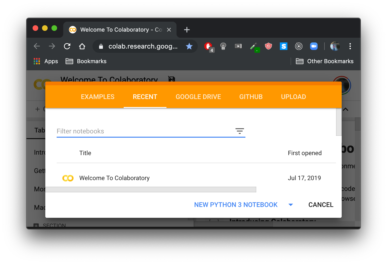
Click NEW PYTHON 3 NOTEBOOK
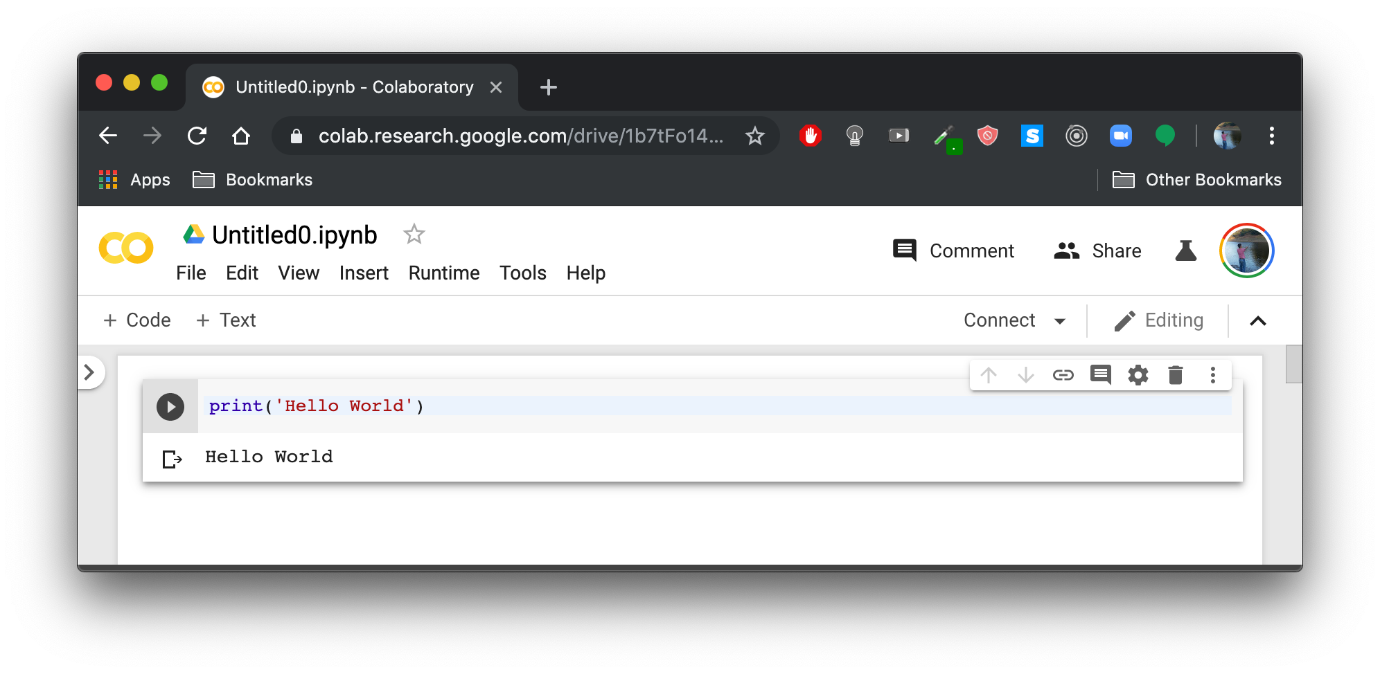
2. You will land on a new Google Colab Notebook:
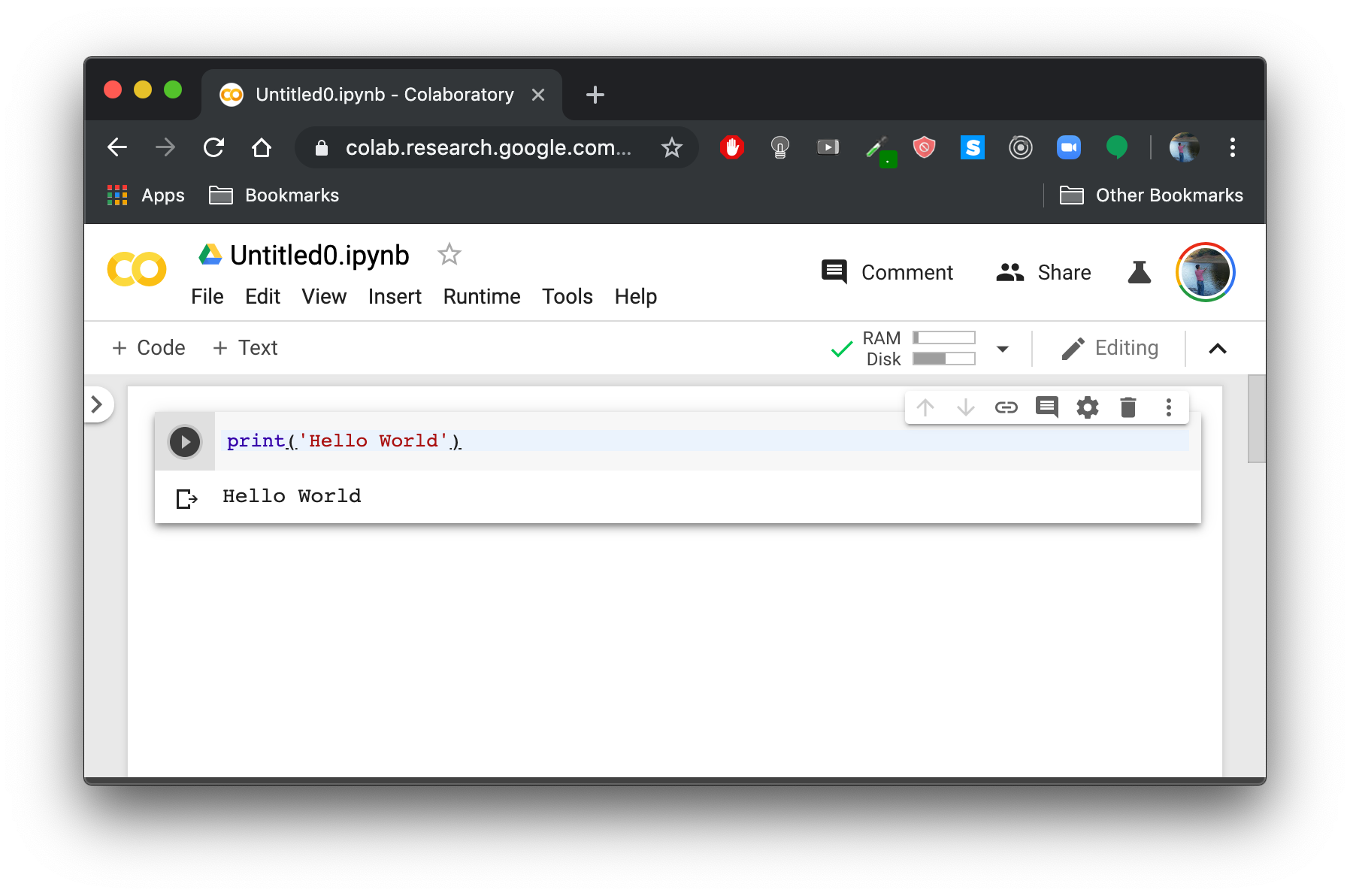
Google Colab Blank Notebook
3. Set up Colab to run on GPU:
Colab offers free use of a Tesla K80 GPU with up to 25Gb of RAM and 12 hours of run-time. It is as simple as going to the Runtime dropdown menu, selecting change runtime type and selecting GPU in the hardware accelerator drop-down menu.
Working with such a large dataset (one-million signals), I found myself running into problems with memory shortages on Colab’s default settings and decided to upgrade to a more powerful Google Cloud Platform virtual machine instance. The one I used costs about 50 cents per hour to run — Just remember to turn it off when you are done training to avoid unnecessary charges.
Note: You can continue along with this tutorial using the free GPU that Colab provides but you may need to train on only a sample of the dataset in order to avoid memory shortages.
Part II: Setting Up a Virtual Machine with GPU
Google Cloud offers a host of cloud-based computing services. I used Google Cloud Platform to run my training session on a virtual machine instance with a Tesla V100 GPU and 50Gb of memory.
Creating a Google Cloud Platform Project
- Go to Google Cloud Platform and click CREATE PROJECT.
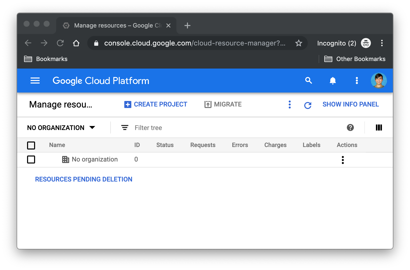
Click CREATE PROJECT
2. Choose a project name and click CREATE.
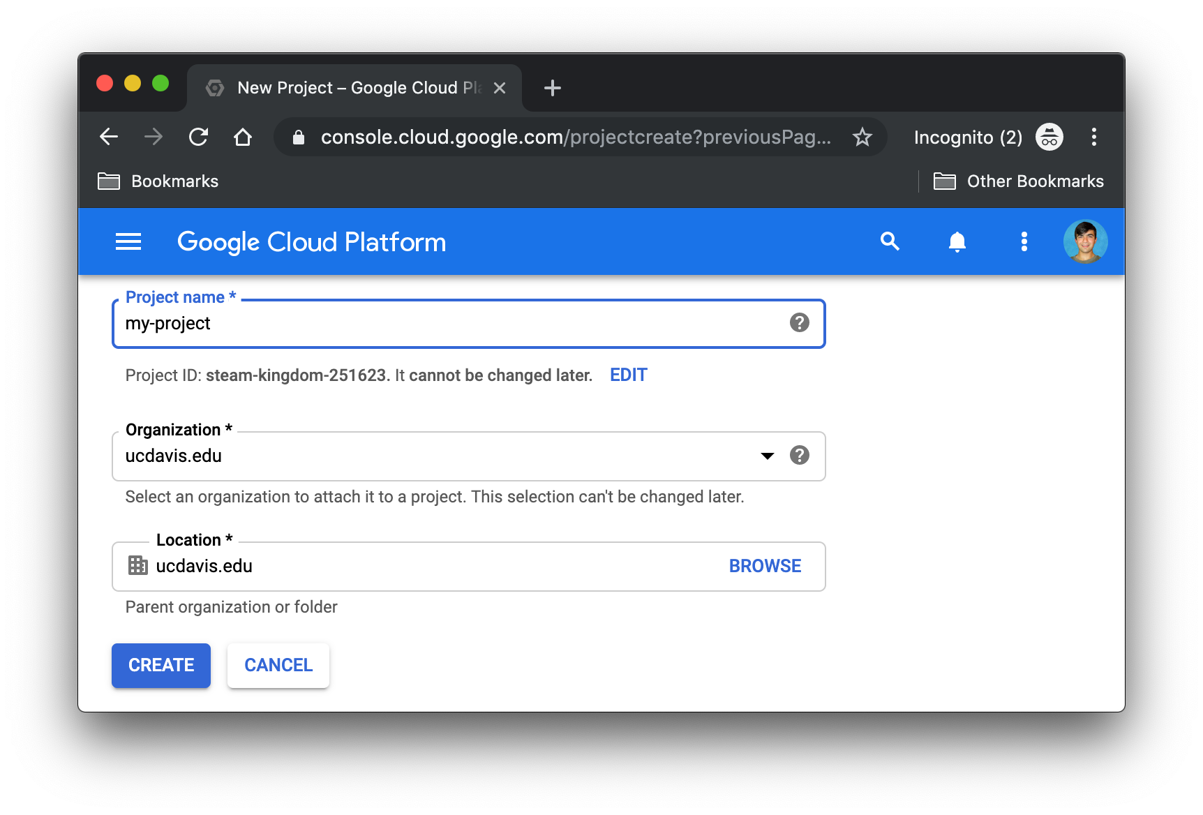
Click CREATE
Creating a Virtual Machine Instance
- Go to Google Cloud’s Deep Learning VM and click LAUNCH ON COMPUTE ENGINE.
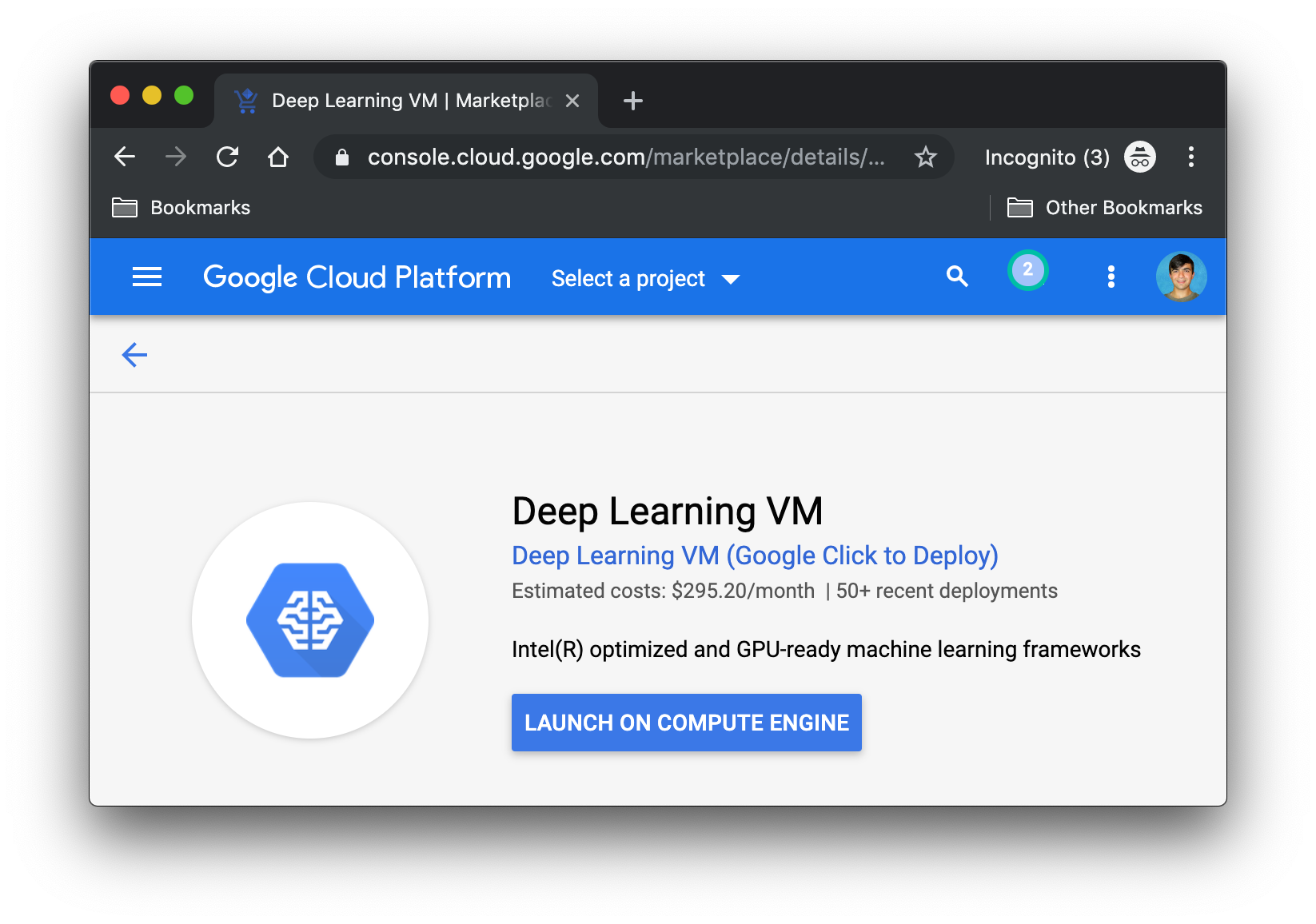
Click LAUNCH ON COMPUTE ENGINE
2. Select your project.
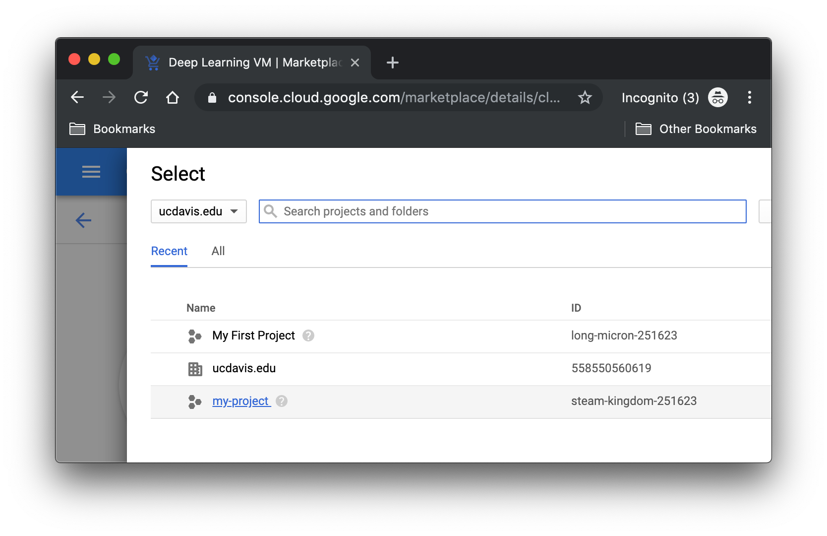
Select your project
Note: First time users will be prompted to enter in their credit card information since this is a paid service. Google currently offers $300 of free credit when you sign up and will not charge you after your credit is used unless you give the OK.
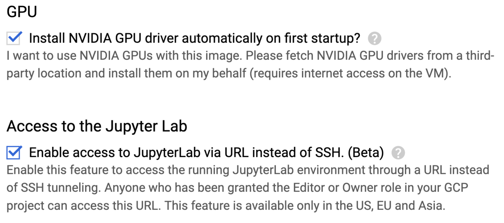
3. You will land on the Deep Learning VM Deployment page. Set your deployment name, choose a GPU type, and make sure the following options are enabled:
4. Accept the terms of service and click Deploy.
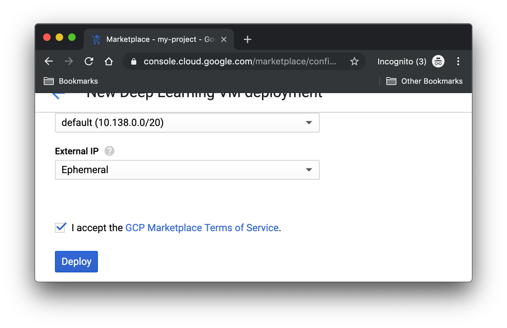
Click Deploy
5. You have successfully deployed a deep learning virtual machine instance! You can check by selecting Compute Engine -> VM Instances.

6. Select your VM instance and click the start button.
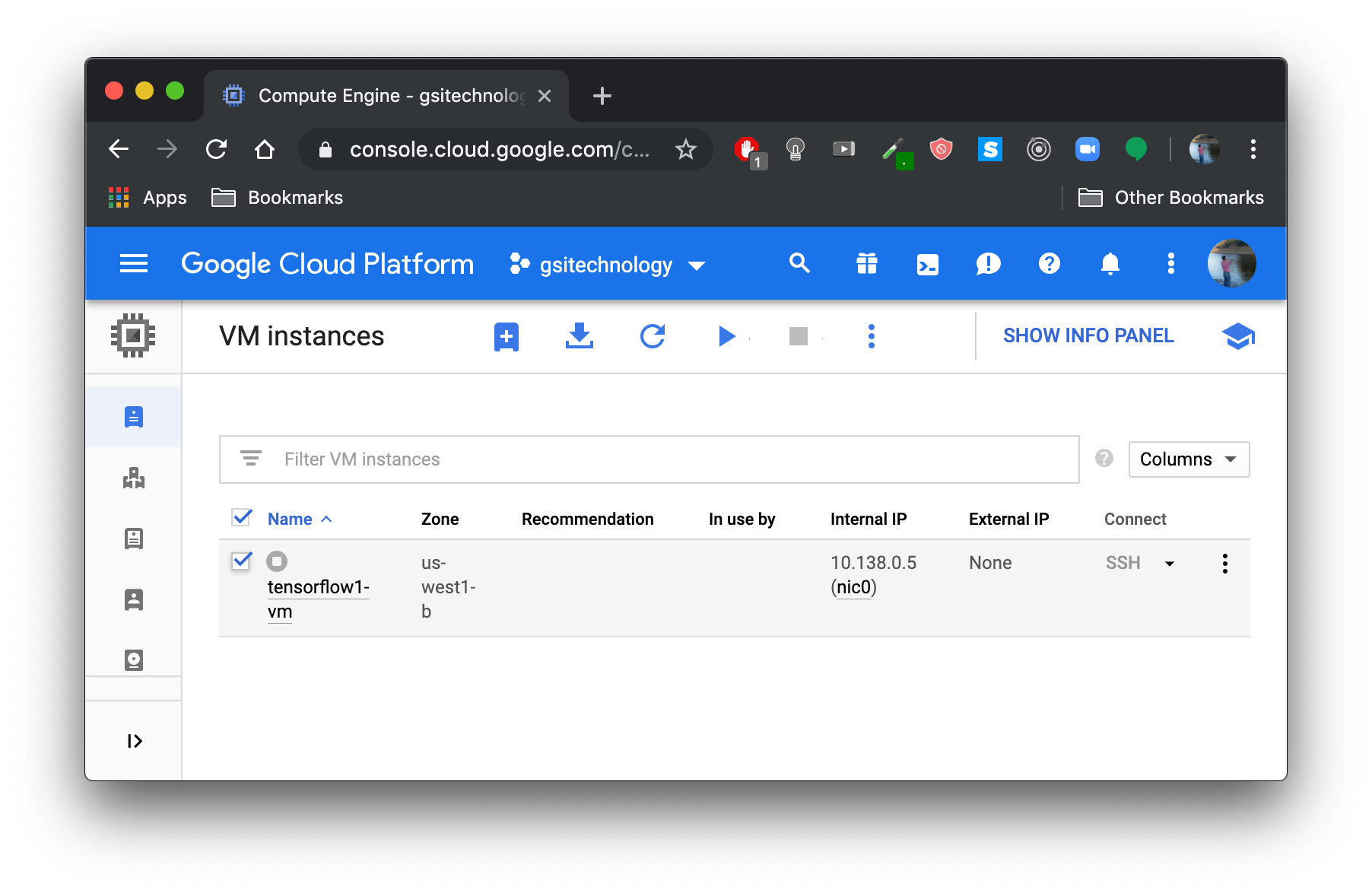
Click START
Your virtual machine is now live. Finally, we will install the gcloud Command-Line tool that will help us remotely access our virtual machine.
Installing the gcloud Command-Line Tool
Google Cloud provides a variety of installation options for different operating systems. I will be showing you the installation process for macOS but you can follow along with one of Google Cloud’s Quickstarts if you are running on a different system.
- Download the archive file.
- Extract the archive file in your home directory.
- Initialize the SDK by running the following command in terminal:
gcloud init
4. Accept the log in option using your Google account: enter Y to accept.
To continue, you must log in. Would you like to log in (Y/n)? Y
5. Log into your Google account when prompted and allow permission to access Google Cloud Platform resources.
6. Back in terminal, you will be prompted to select your Cloud Platform project. Choose the project you created. If you only have one project, you can skip this step.
7. Select a default Compute Engine zone.
8. Run gcloud init in the command line to verify you completed all steps successfully:
gcloud init
Done! — gcloud has been installed and we are ready to access our virtual machine.
Accessing Your Virtual Machine
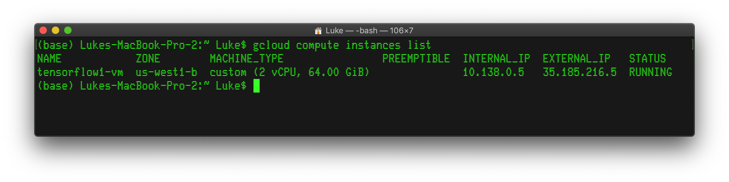
- In terminal, view your VM instance information by running:
gcloud compute instances list
Your unique instance information will be displayed as follows:
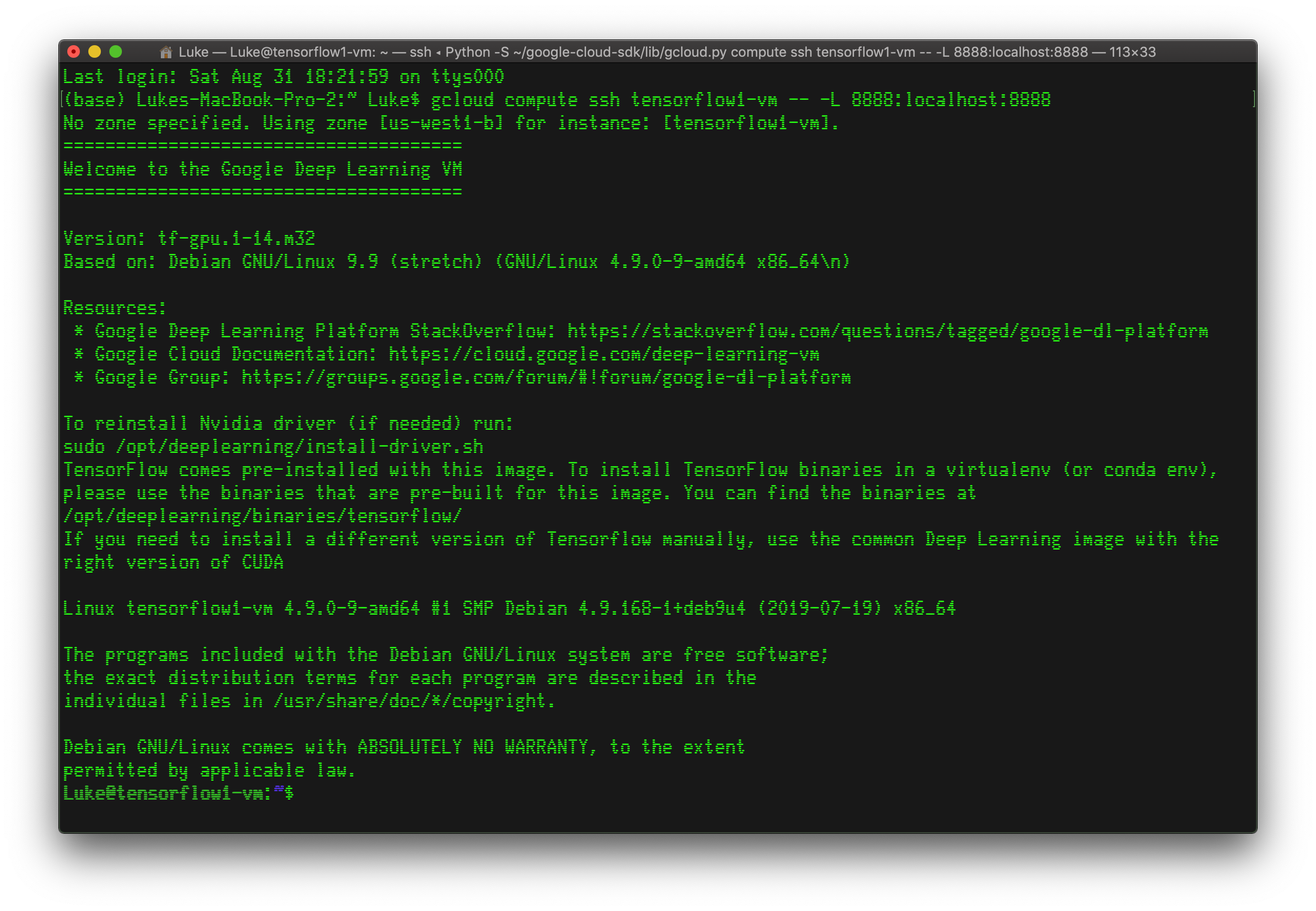
2. ssh into your virtual machine with the following command (make sure to use your unique instance name):
gcloud compute ssh <instance-name> -- -L 8888:localhost:8888

3. You are remotely connected to your virtual machine!
4. Run the following command to see your VM GPU information:
nvidia-smi

GPU Information
I am running on the Tesla V100 GPU (same as described in the paper). Your GPU type may differ depending on how you configured your deep learning virtual machine.
Part III: Connecting Colab to Your Virtual Machine
Almost there!
Now all that is left is to connect the virtual machine we just created with our Colab Notebook.
- Run the following code in your virtual machine command line:
jupyter notebook \
  --NotebookApp.allow_origin='https://colab.research.google.com' \
  --port=8888 \
  --NotebookApp.port_retries=0
This will allow your Google Colab to access your virtual machine.
2. Go back to the Colab Notebook you created earlier in your browser.
Colab Notebook
3. Select Connect to a local runtime in the Connect dropdown menu.
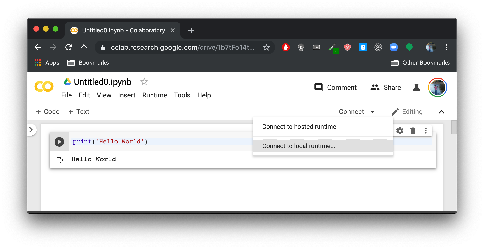
Connect to local runtime
4. Enter backend port: 8888 and click CONNECT.
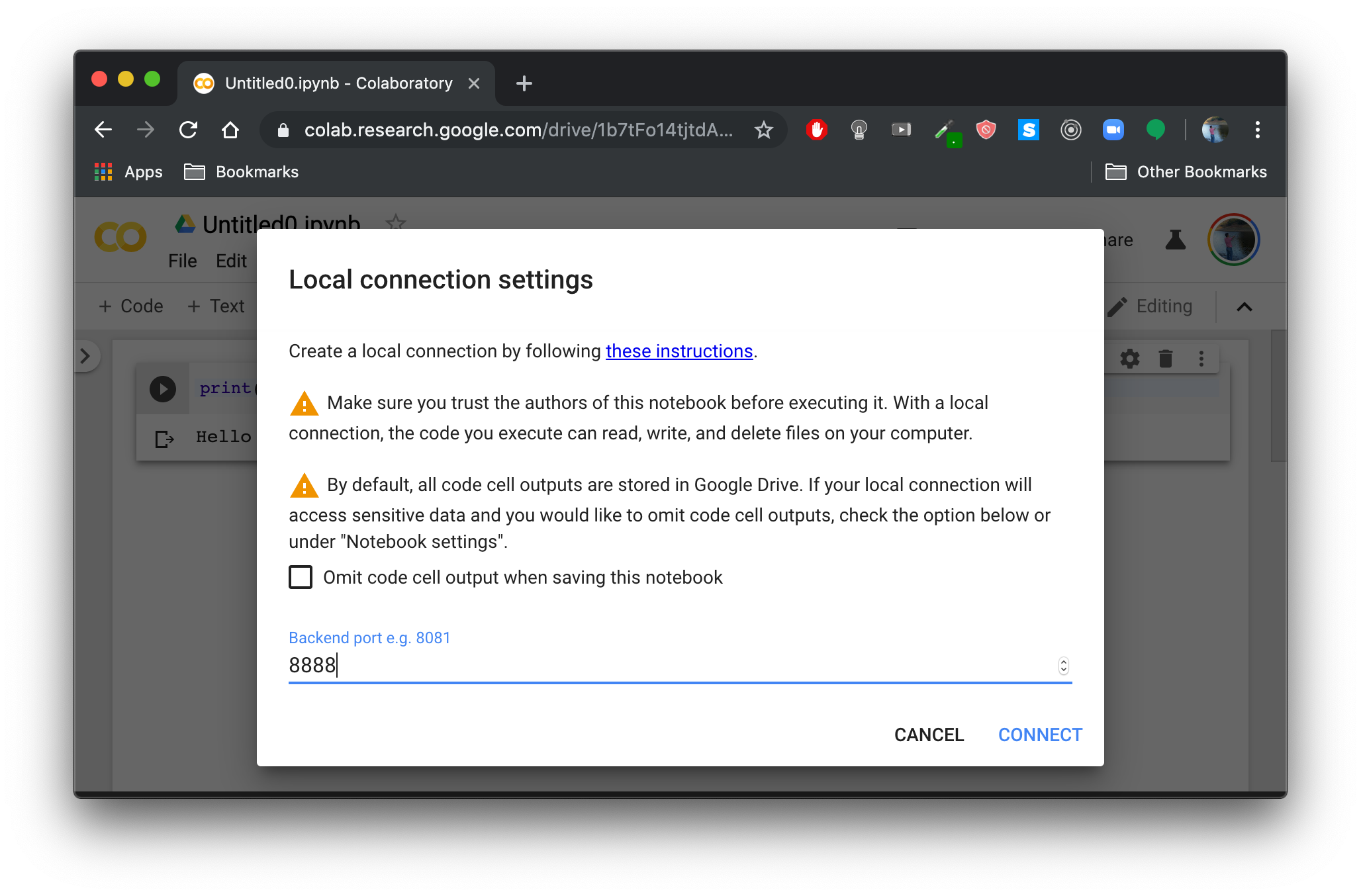
Backend port selection
5. Done! Your Colab notebook is now connected to your virtual machine.
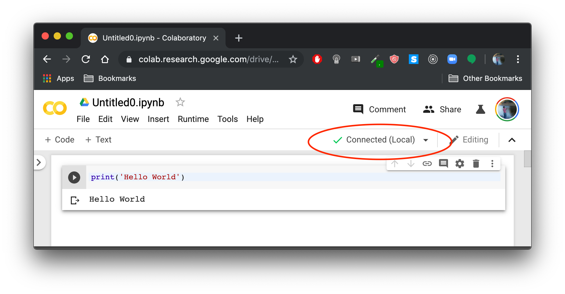
Colab connected to virtual machine
Now any code you run in your Colab Notebook will be running on your virtual machine’s accelerated hardware. This will be very useful later, as traditional hardware takes much longer to train large networks with lots of data.
Ready to Start Coding
Finally, the fun part! We are now ready to start coding a ResNet in Python.
Part IV: Coding a ResNet in Python with Keras
Before We Begin
We will now walk through a step by step process of building a ResNet in Python. If you want to look at the code in its entirety, here is a link to my Google Colab: ResNet Signal Classifier Notebook.
Colab offers a cool feature called Playground which will allow you to edit and and execute the ResNet code from my Notebook directly within your browser:

Edit and execute
You will, however, be required to download the dataset (described in next section) in order for this to work.

Keras: The Python Deep Learning Library
Keras is a high-level neural networks API that is capable of running on top of Tensorflow as well as several other machine learning frameworks. Keras is developed with a focus on enabling fast-experimentation, simplifying the process of building neural networks and testing models.
If you are a first-time Keras user but relatively familiar with deep learning concepts, you should still be able to follow along with the code without too much trouble. However, I recommend brushing up on Keras’ functional API before we dive in.
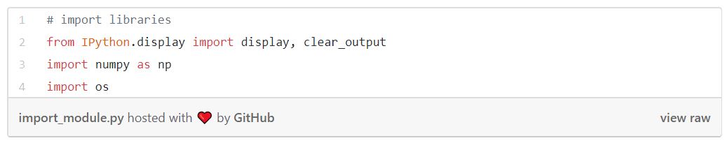
Importing Libraries
Create a new cell in your Colab Notebook and enter the following code to import all necessary modules:
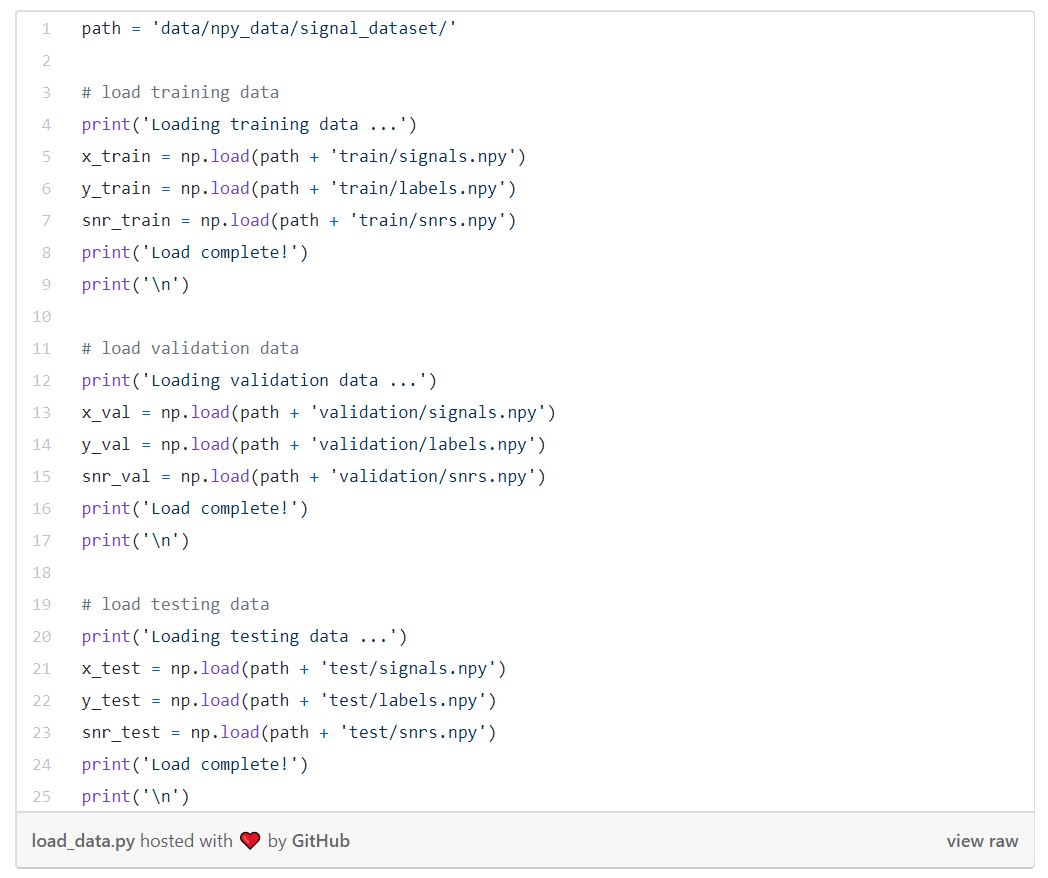
Getting and Loading the Data
The original dataset from Deepsig.io comes in .hdf5 format. I converted the data to .npy format since I found it took much less time to load. The signals are divided into training, testing, and validation data. Here are links to a small and large dataset of labeled signals:
Download Link: Dataset (9.1GB)
Once downloaded, you can transfer the dataset from your local computer to your Google cloud instance by using the command:
gcloud compute scp dataset.zip <instance-name>:~
Back in your Colab notebook, create a new cell and enter the following Python code to load the dataset .npy files. Just be sure to adjust the path variable according to where the data is located on your machine.
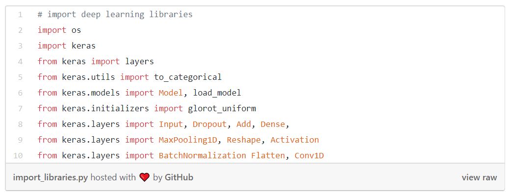
Import Deep Learning Libraries
These are all the functions from Keras that you will need to make your ResNet. Add this code to a new cell in your Colab Notebook.
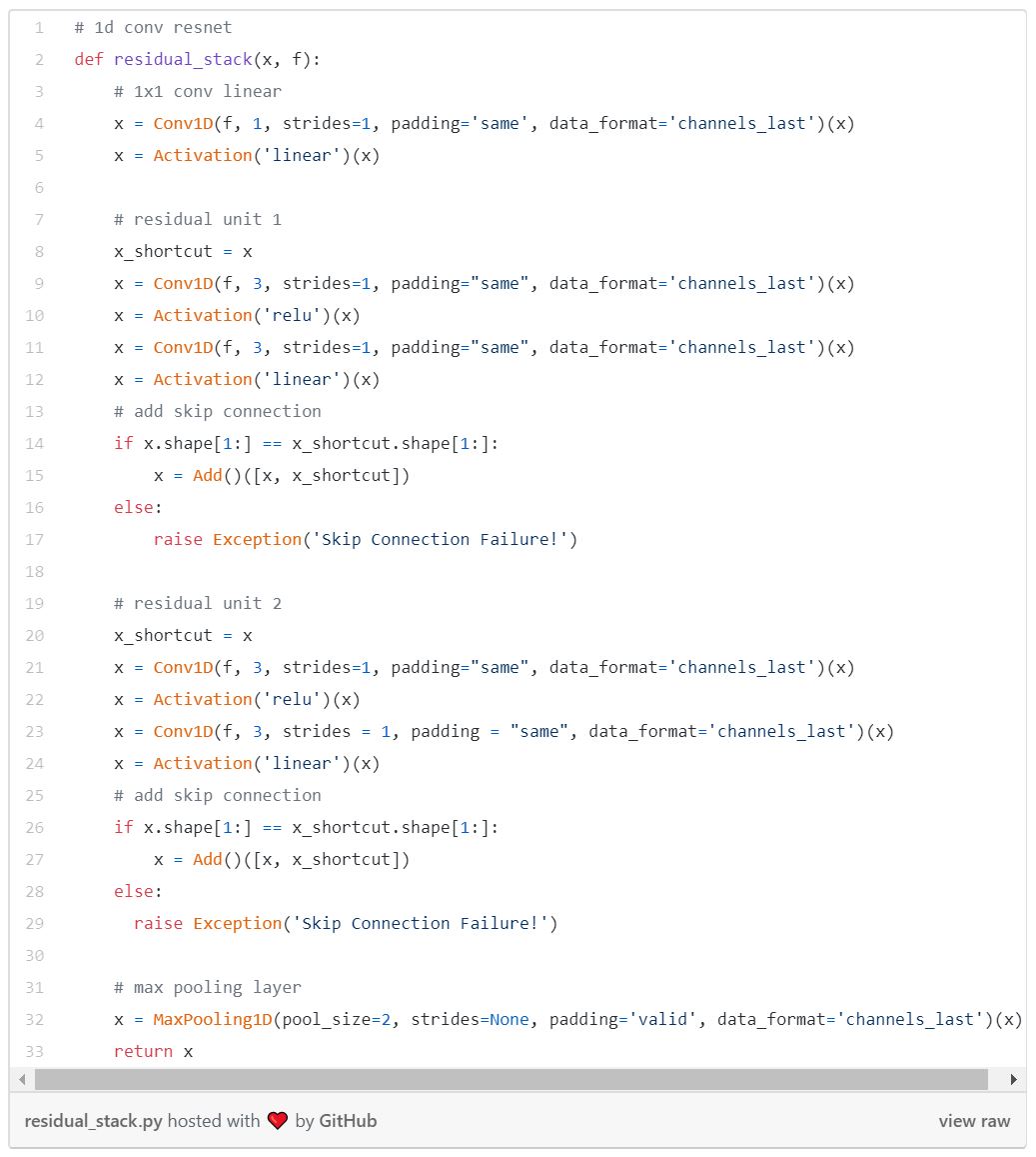
The Residual Stack
This is the part of the network that makes the neural network a residual neural network. Notice how x_shortcut saves the state of x and gets added back in after (or skips) two convolutional layers — this is the skip connection.
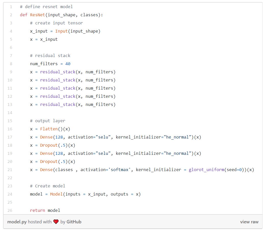
Define the Model
We add five residual stacks and two dense layers with dropout for regularization. The final layer is the output of classification probabilities.
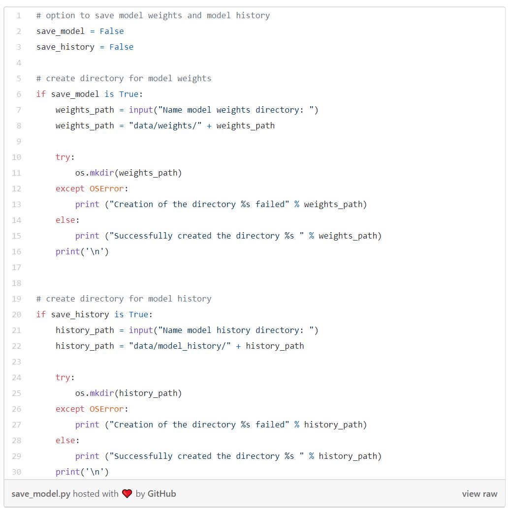
Add Option to Save Model
If you want to save the model weights and history, include the following code in a new cell and set save_model and save_history to True.
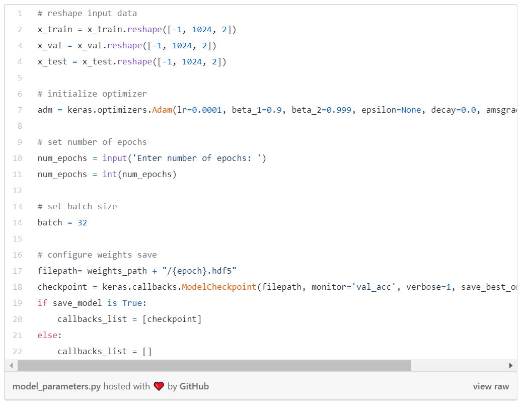
Set Model Parameters and Reshape Data
Here we set the optimizer, learning rate, batch size, number of epochs, and reshape the data into a format that Keras can process.
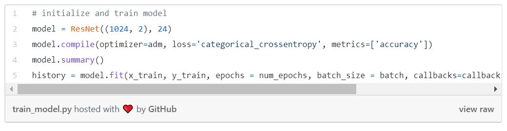
Initialize and Train Model
Finally, we initialize the model and use model.fit() to train the network. Keras has a convenient summary feature that gives you high level information about your model. This model has 287,056 trainable parameters.
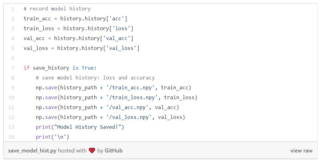
Save Model History (Optional)
If you would like to save the model accuracy and loss information from every training epoch, enter the following code in a new cell:
Run the Code and Train the Model
That’s it! Now you can run the code within the Notebook and start training your model. I trained my model on 1.2 million signals for 100 epochs. This required about 15 hours of training time on my Tesla V100 GPU — I left it running over night and came back to it the next day …
Evaluate the Model
The model achieved an overall accuracy of 96.4% on the high SNR testing data* (compare to accuracy reported in the paper of 99.7%). Just short of the paper by 3.3%.
The graph below shows the overall model accuracy by SNR. For SNR 10 and higher, the model shows very reliable performance. As expected, the more interference a signal has, the more difficult it is to accurately classify.
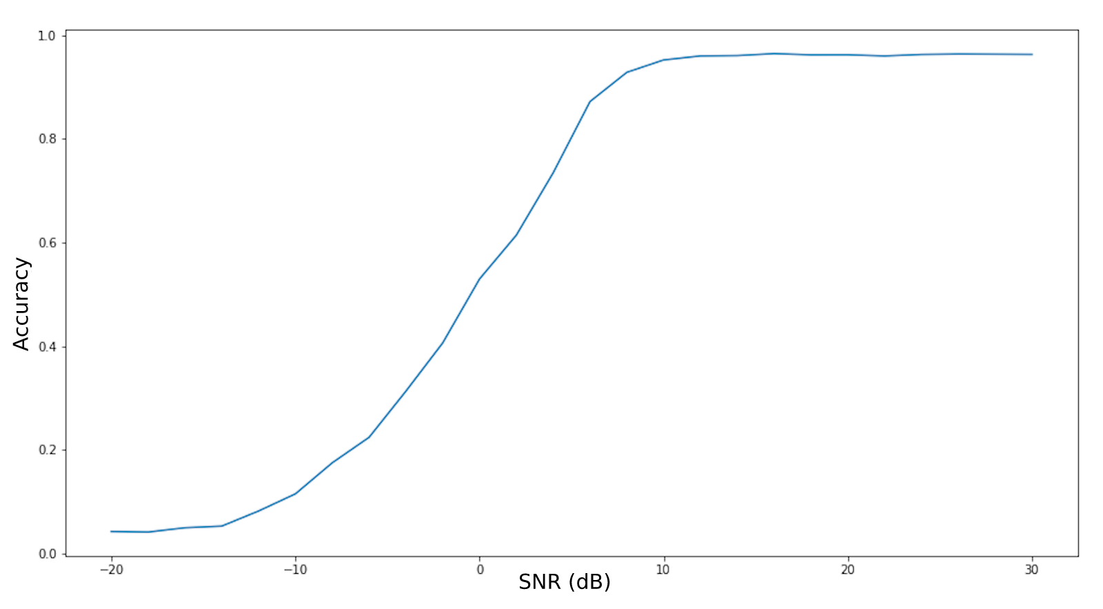
Model Accuracy by SNR
Here is a graph of the overall performance of the model on a testing dataset of both dirty and clean signals by epoch.
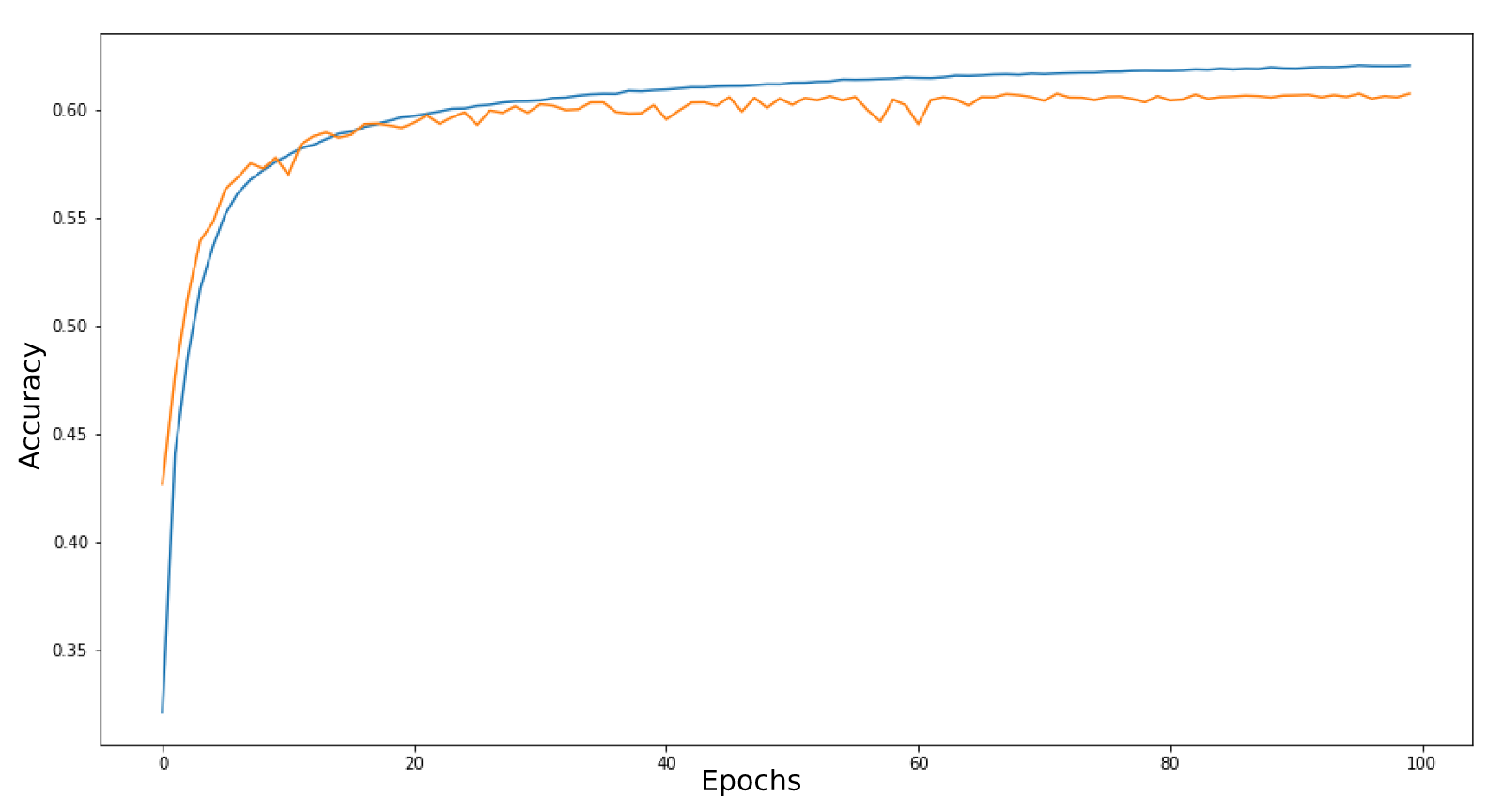
Model Accuracy by Epoch
The blue line represents the training data and the orange line represents the validation data. The model learns very quickly within the first 10 epochs and then makes slow but consistent gains until learning plateaus. Note that the graph shows a maximum classification accuracy of 60% — this is because the model is being tested to its absolute limits on a mix of clean signals and signals with very high interference. Some of the signals have so much noise that they are virtually unrecognizable.
Reaching a maximum accuracy of 96.4% on the clean signal dataset, the model is, of course, not perfect. Here is an example of a signal that was mis-classified by the model; this particular AM-DSB-SC signal (top) was mis-classified as a 128QAM signal (typical example seen on bottom).
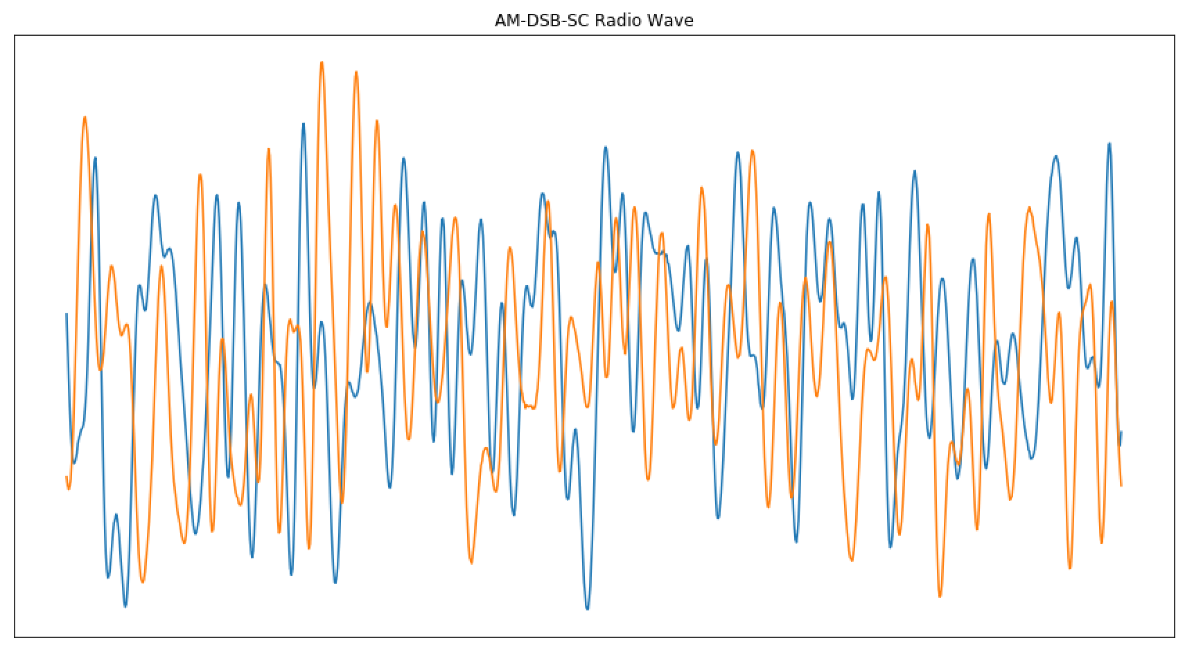
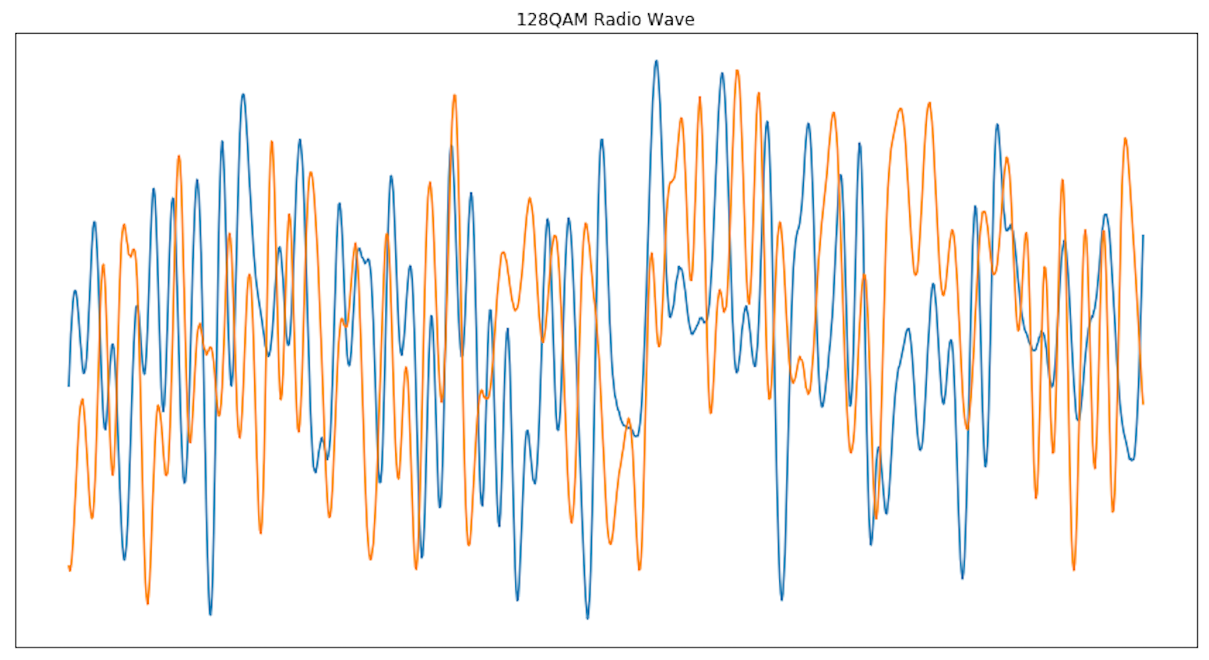
AM-DSB-SC signal (top) mis-identified as 128QAM signal (bottom)
It is easy to confuse AM-DSB-SC and 128QAM signals since they are so similar. Even to the trained eye, these signals may be difficult to tell apart.
Here is a download link to the weights for the model that I trained. If you don’t want to spend time training your own model but would still like to test the signal classifier, you can simply load the provided weights and try testing out some signal examples. Here is a link to a tutorial for loading weights in Keras in case you get stuck: How to Load a Keras Model.
Conclusion
Based on this work, we can say for certain that deep learning does show promising results for signal classification.
Now that we have a deep learning model to classify signals we can use the model to extract embeddings for signals. This is useful because, as we will see in the next blog, we can reframe signal classification as a similarity search problem. In the next blog we will modify the model to learn fingerprints that can be used in a similarity search database.