Introduction
In my last blog, I introduced RDKit and Tanimoto similarity. In this blog, I will introduce another similarity search technique based on mol2vec. But first, let’s talk about word2vec.
Intro to Word2vec
Word2vec is one Natural Language Processing (NLP) technique that allows you to treat words and sentences as numbers. This is useful for many things, such as determining similarities between words and documents. The image below shows an example of word2vec.
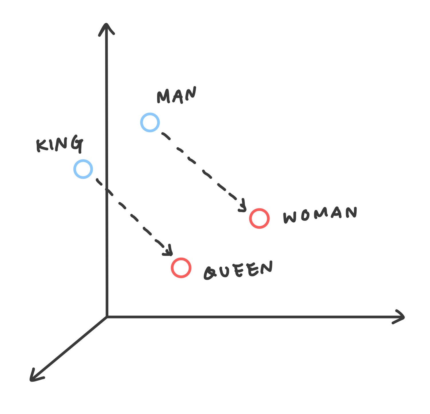
Since word2vec transforms words into vectors, it allows us to perform mathematical operations. The image above is the famous example of
king - man = queen — woman.
Mol2vec
Molecules can be translated into vectors too! Here is an animation of a plot that shows substructures are grouped based on their similarity:

Each blue dot represents a molecule in the vector space. As the cursor moved to the molecules intersection, we can see that the similarity of the substructure is maintained in the vector space. On the other hand, the substructure of the molecule that is located farther away looks dissimilar. Note that the number on each molecule is the Morgan fingerprint of the substructure highlighted in green.
Isn’t that cool? But how do we get this? To translate molecules to vectors, we first need to understand an advanced cheminformatics concept — Morgan fingerprints.
Morgan Fingerprints
A Morgan fingerprint is just a numeric identifier for a molecule substructure. They are designed for molecular characterization, similarity searching, and structure-activity modeling. These fingerprints are an effective and popular search tool that can be applied to a wide range of applications such as drug discovery.
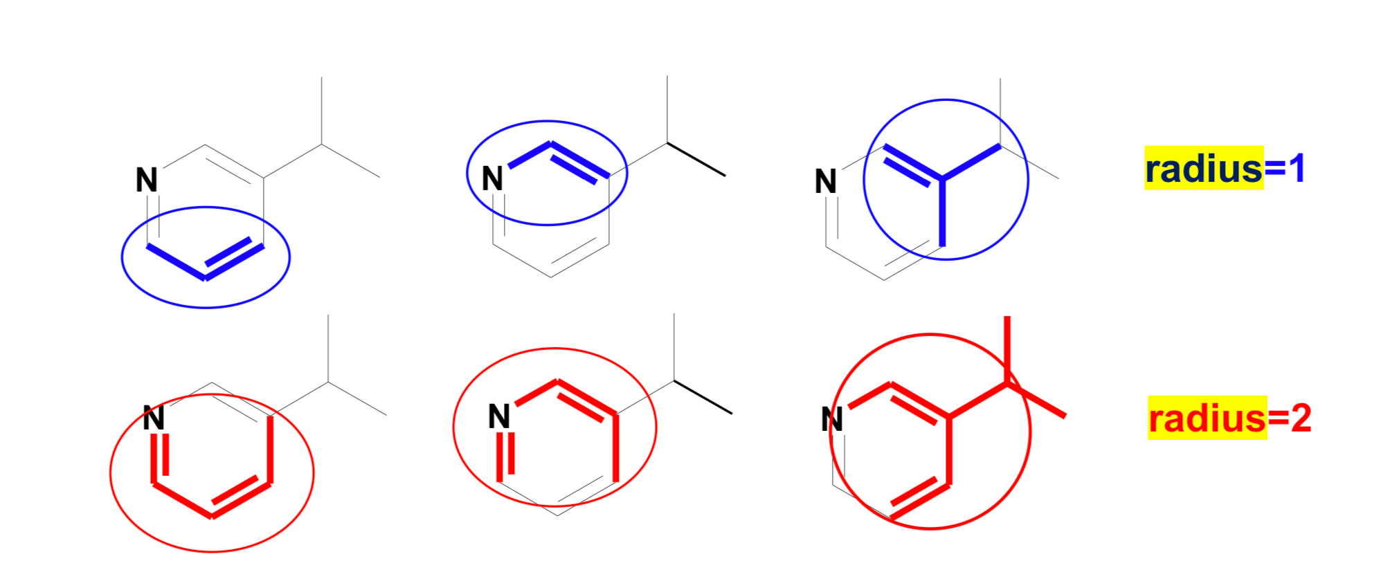
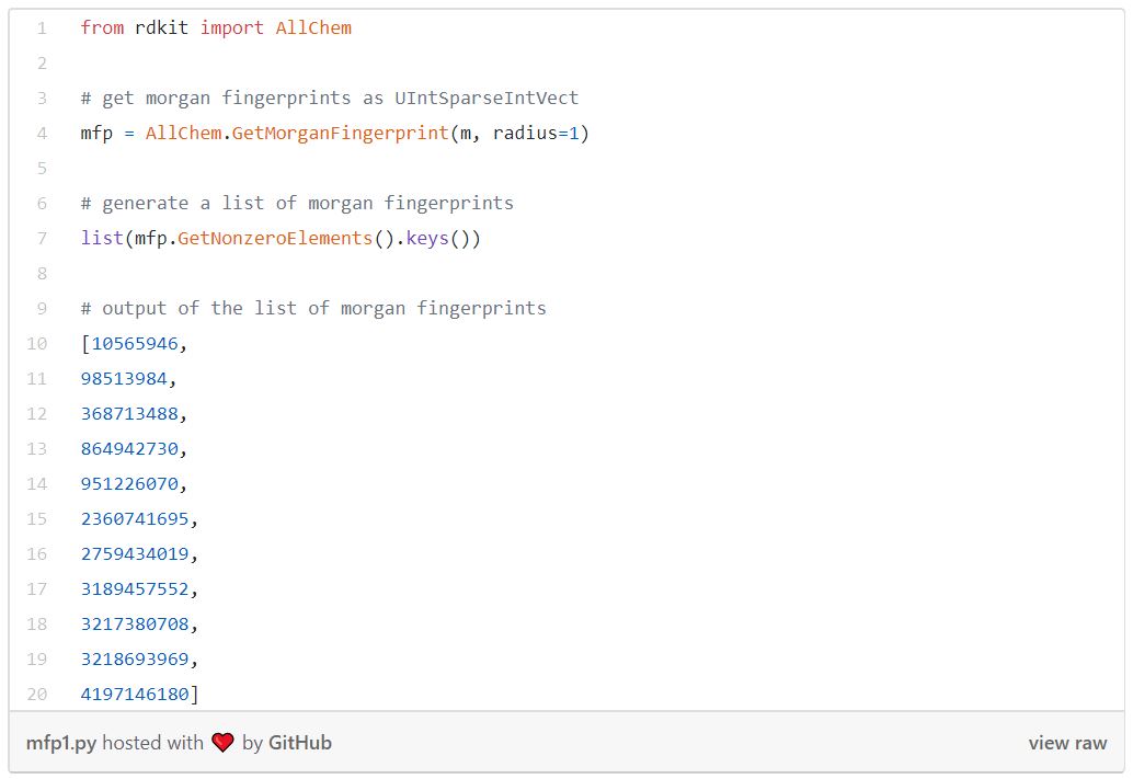
There are straightforward RDKit functions that generate Morgan fingerprints. They take a molecule, a radius, and some other parameters. But here, let’s talk a little bit more about radius. Radius is the neighborhood of each atom, as shown in the image below, so if
♦ radius = 1: it is one bond away from the atom
♦ radius = 2: it is two bonds away from the atom
♦ and so on…
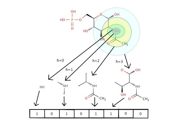
Each substructure is associated with a bit in a bit vector. In practice, these bit vectors can be very long; sometimes they can get up to 8Kb. In RDKit you can retrieve Morgan fingerprints as bit vectors or shorter integer identifiers.
Mol2vec uses Morgan fingerprints to compose molecule vectors.
The Mol2vec Project
While I was trying to look for examples of converting molecules into vectors, I found this paper and a Github repository of mol2vec. After learning about what the mol2vec project is about, I started doing experiments on the ChEMBL database using the mol2vec repository (I showed how to load the ChEMBL database in the last blog.)
The following code is loading a lookup database of molecule vectors in which Morgan fingerprints are the lookup keys. The file can be found inside the mol2vec repository.

As a data scientist, it is always important to make sure the database is cleaned before using. One thing to notice here is that some molecules in the database are Null values; they must be removed in order to proceed with the experiments. Another thing to be careful of is that some substructures do not exist in the model, so checking for the existence of the substructures is necessary.
Vectorizing A Molecule
Now that we’ve loaded all the files we need and cleaned the database, let’s try to vectorize a molecule. The concept is very easy. We first extract all the substructures from the molecule, loop through the model with the corresponding vector, and finally, we add them all up. But there are many ways to combine substructure vectors to get an overall molecule vector, just like combining words in word2vec.
While I was studying all the functions needed, I noticed that RDKit output duplicates of substructures. So then I decided to do experiments on duplicates and unique. I also did experiments on averaging the vectors to normalize them. The results will be presented later in this post. Here is the list of all combinations I’ve tried:
♦ Duplicates: add up all substructures outputted by RDKit
♦ Unique: add up only the unique set of outputs
♦ Average Duplicates: average the summed vector of duplicates
♦ Average Unique: average the summed vector of unique
The following is the function of duplicates.
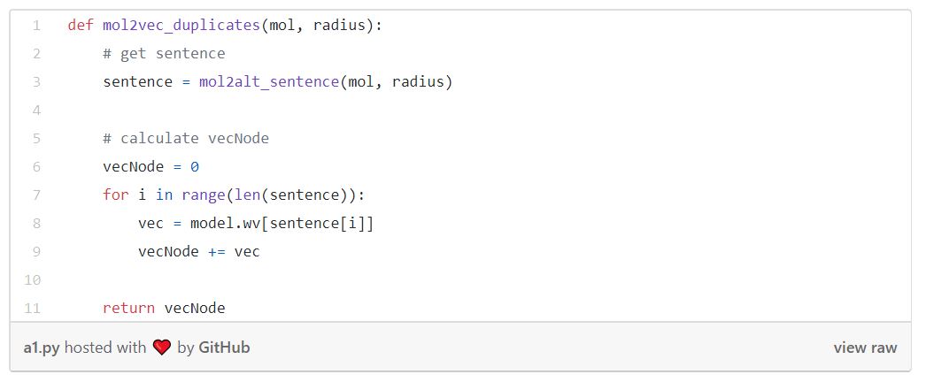
Other algorithms are similar to the one above, but with a slight difference.
Similarity Distances
After converting molecules into vectors, let’s compute the similarity distance. Here I used Euclidean distance and cosine distance. The following image depicts the difference between Euclidean and cosine distances.

Difference between Euclidean and cosine distances
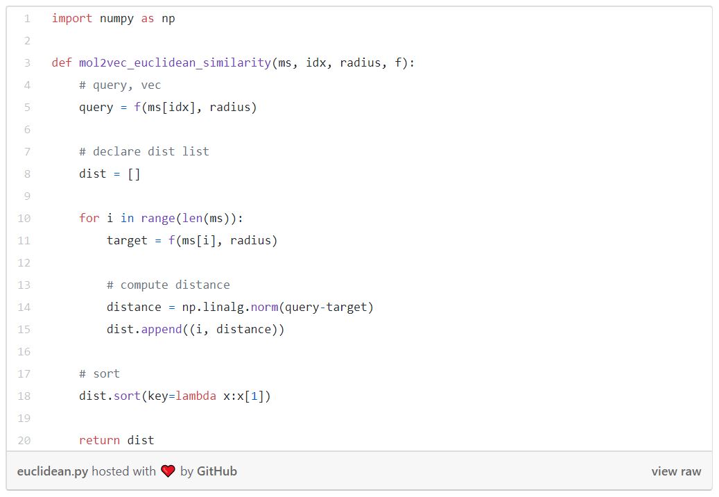
The function below is computing Euclidean similarity between the query and all the molecules in the database.
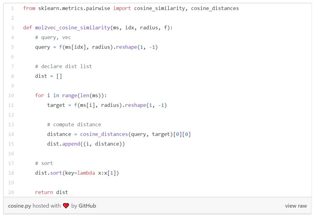
And this one is computing the cosine similarity.
Euclidean vs Cosine
Since I am treating the Tanimoto similarity as the ground truth, I will be comparing it against Euclidean and cosine similarities. Here I am using the technique of recall@K, meaning finding the K nearest similarity.
Now let’s visualize the experiments. I will be showing the results of sample sizes of 100 and 1000 from the ChEMBL database, which has a total size of 440055, and a query size of 20. In my experiments, I used k= 1, 5, 10 to calculate the recalls because when using k= 1, we can easily determine whether these techniques give the same nearest neighbors as Tanimoto similarity.
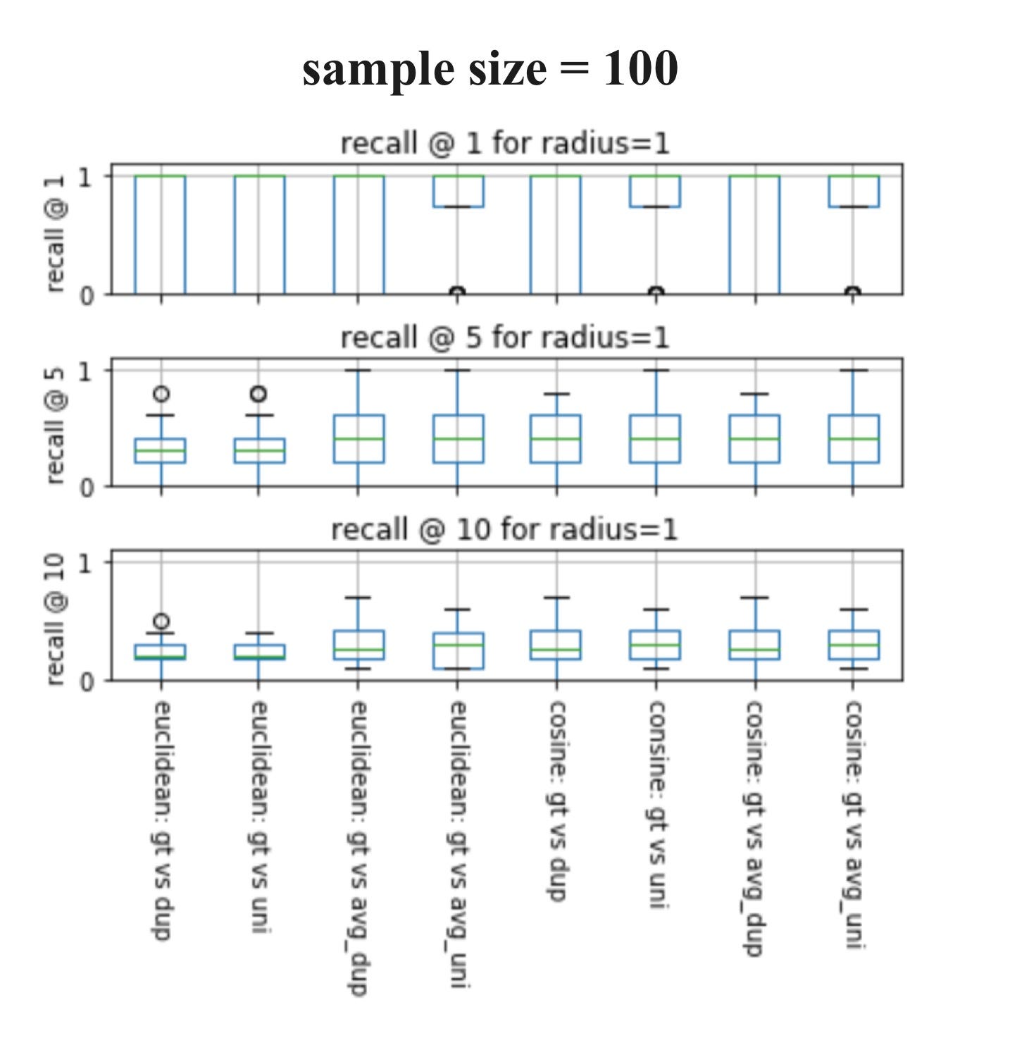
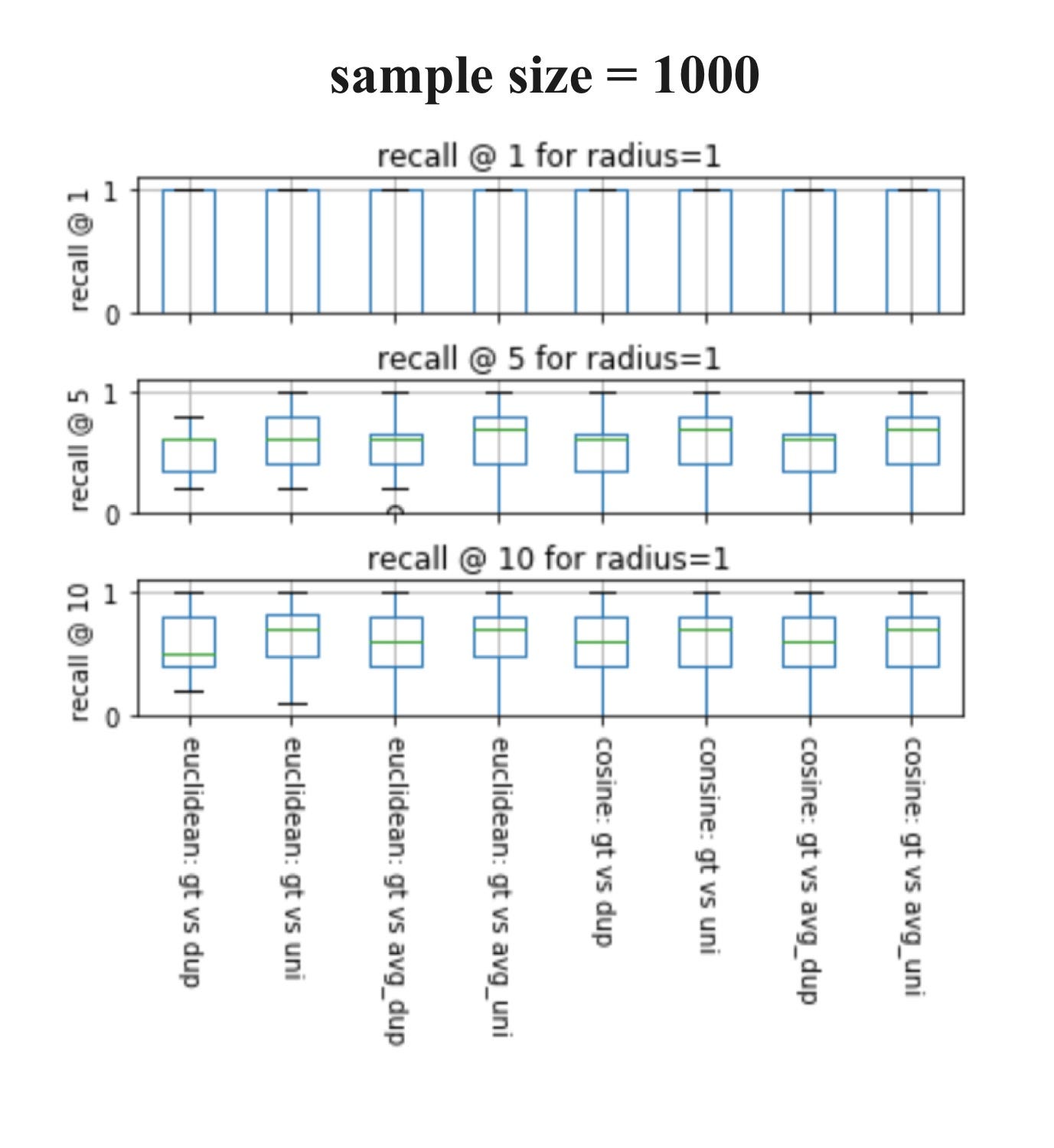
If you’ve never seen a box plot, it’s a very simple concept. We use them to visualize in one place the descriptive statistics for a set of experiments. This includes median, spread, and outliers.
Here are some observations:
♦ When sample size= 1000 and k= 1, all eight techniques always result in the same nearest neighbor as Tanimoto.
♦ As both box plots above show, we can generally conclude that when sample size increases, recall increases for all k.
So which technique has the best performance? The line graph below shows the top 4 techniques when k= 10 (Note that some data points overlap.)
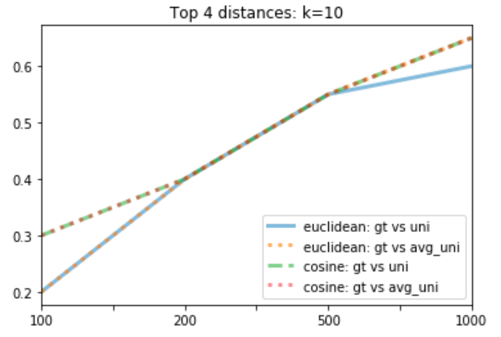
The line graph above shows that both cosine distances have the same performance, which is the best out of the 4.
Conclusion
In conclusion, I’ve found that the mol2vec similarity is very close to Tanimoto similarity. For example, look at the image below — I showed the top 10 using Tanimoto and cosine unique for one query, which is the left most molecule:
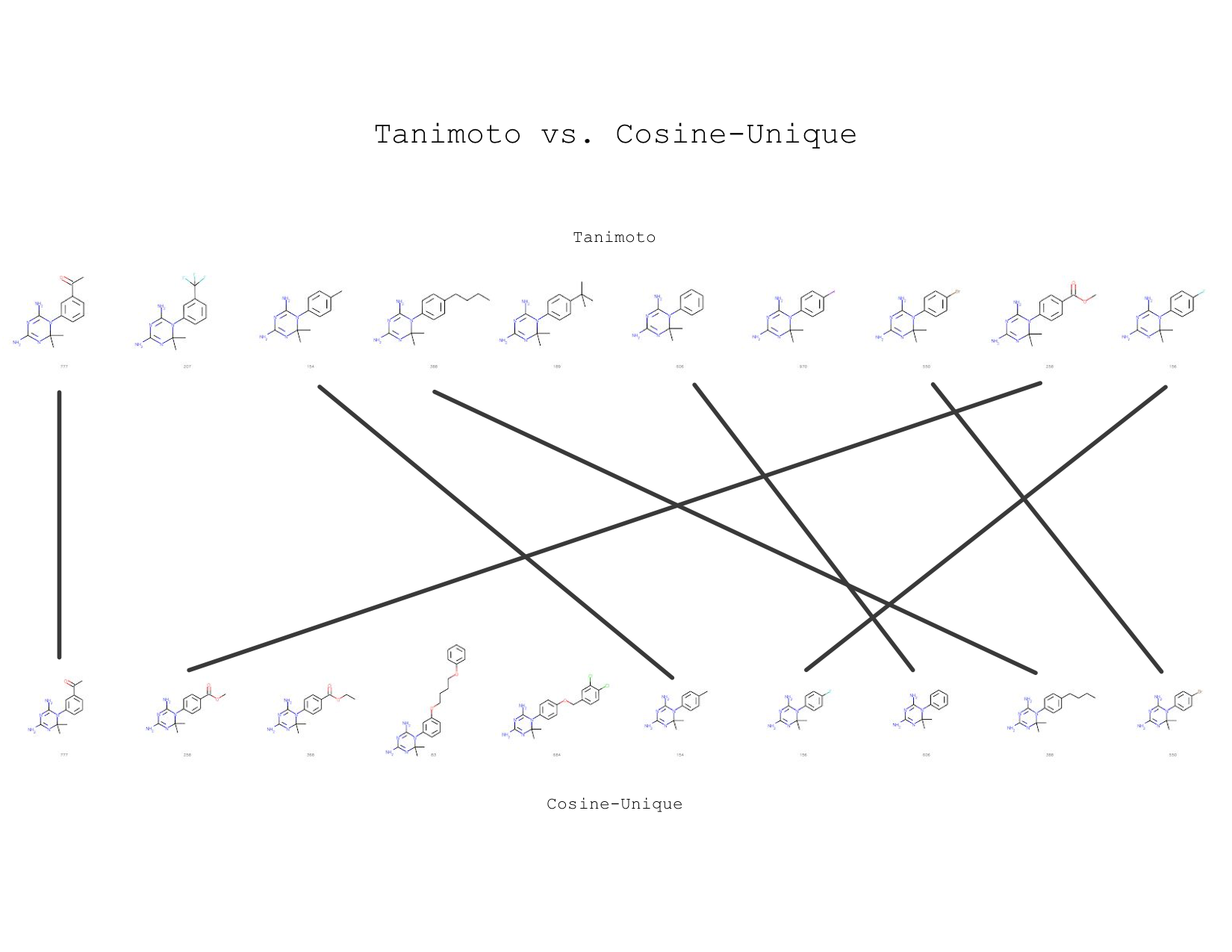
Nearest neighbors are ranked from left to right, query is the first molecule
Notice that 7 out of 10 nearest neighbors are also in the Tanimoto neighborhood. It’s very cool to see how two molecule similarity search techniques can yield nearly the same result!
For the follow-up work, we are considering trying the following:
♦ Different distance functions, including Dice, Sokal, Russel
♦ Training our own model based on ChEMBL databases
♦ Transfer learning on pre-trained mol2vec models